Stumbling Distance

We have the two components of our drinkiness model: geographic data (where the bars are) and temporal data (when rides happen). The task is to combine them: for each taxi ride, calculate how “drinky” the pickup location and time are.

The time component is straightforward. The location component is where things get interesting — and where we’ll nearly break the laws of computational feasibility.

The Drinkiness Clock

First, the easy part. We need to assign a drinkiness weight to each hour of each day of the week.

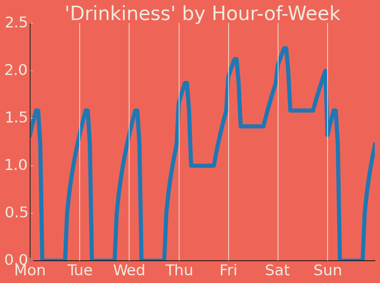
This is admittedly the most subjective part of the analysis. I consulted with current and former New York City denizens, toyed with the idea of a Survey Monkey poll, and ultimately went with expert judgment — which is a diplomatic way of saying “my own informed guesswork, refined by arguing with friends.”

The basic logic:

• Drinking ramps up toward the end of the week
• Drinking ramps up through each evening
• A weekend afternoon has some drinking, a weekday evening has more, and a weekend evening has the most of all
• The dead zone is weekday mornings — not zero, because this is New York, but close

Mapping each taxi ride’s pickup time to this model gives us a temporal drinkiness score. The hard part comes next.

The Spatial Problem

For each taxi ride, we need to answer: how many bars are within stumbling distance of the pickup, and how strong are they?

This requires a notion of distance. The heatmap from earlier assumed that a bar’s influence radiates outward evenly in all directions — a circle. Mathematically, that’s the L2 norm (Euclidean distance). It means a person could stumble straight through buildings, over the East River, or across Central Park. Technically possible after enough drinks, but not a great assumption.

A better choice might be the L1 norm, also known as the Manhattan distance — or, coincidentally, the taxicab distance. This restricts movement to a grid aligned with the compass directions, which is closer to reality in Manhattan’s street grid. But it still doesn’t account for actual street layout — diagonal streets, dead ends, parks, rivers, that inexplicable block in the West Village where the streets stop making sense.

What we really want is a stumbling distance norm: the walking distance along streets, ignoring traffic restrictions like one-way signs, because a drunk person is not going to let a traffic arrow dictate their route home.

The Naive Approach (1,068,054 Years)

To calculate stumbling distance, we need routing. Google Maps has a convenient directions API — you give it two points, it gives you a walking route and distance.

Let’s do some quick math:

11,000 bars × 88,600,000 rides = 974,600,000,000 routing requests

Google Maps API allows 2,500 direction requests per 24-hour period.

974,600,000,000 ÷ 2,500 = 389,840,000 days ≈ 1,068,054 years

We can get this done in just over a million years. I informed Steve that we might need to extend the project timeline.

Building Our Own Router

There are certainly excellent commercial GIS products out there, but the whole point of this exercise is to use free tools and run everything on a laptop. With freely available shapefiles (at the time, Mapzen offered excellent metro extracts; they’ve since shut down, but OpenStreetMap exports fill the same role) and Python mapping libraries, we can build our own router.

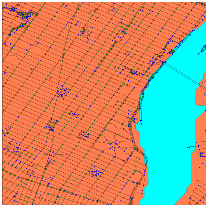
The key insight: streets are a graph. Each intersection is a node, and each street segment is an edge. Shortest-path algorithms (Dijkstra’s, A*) are well-understood and fast on graphs of this size.

The shapefile defines streets as line segments, but doesn’t explicitly identify intersections. We solve this by computing them geometrically — finding where street segments cross each other. The green dots in the image above are intersections we discovered this way. Once we have the graph, shortest-path routing is straightforward.

By doing our own routing, we eliminate the API rate limit entirely. But 88.6 million rides against even a handful of nearby bars is still a mountain of shortest-path calculations. We need to be smarter about which bars to check for each ride.

Making It Fast: k-d Trees

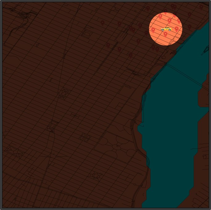
Enter the k-d tree (and its cousin, the ball tree) — spatial data structures designed for efficiently finding nearest neighbors. Instead of checking every ride against every bar, we pre-index the bar locations into a k-d tree. Then for each ride, we query “what bars are within radius R?” and get back just the handful of nearby ones.

These data structures are used under the hood in many spatial APIs for nearest-neighbor searches. They’re especially powerful when you need to find nearest neighbors over and over — which is exactly our situation.

The key subtlety: we use Euclidean distance for the k-d tree radius search, not stumbling distance. Why? Because Euclidean distance is always less than or equal to walking distance (a straight line is always shorter than any path along streets). So the Euclidean radius gives us a conservative superset of the bars that could possibly be within stumbling range. We then compute the actual stumbling distance only for that small subset.

This two-stage approach — fast approximate filter, then precise calculation — is a common and powerful pattern in spatial algorithms.

The Final Optimization

One more trick: many taxi rides start from very similar locations. Two rides that both originate near the corner of 7th Avenue and Christopher Street don’t need independent drinkiness calculations — they’re going to get the same answer.

If we round each pickup coordinate to a reasonable precision (roughly the nearest 50 meters), we can cache the drinkiness score for each grid cell and reuse it for all rides starting from that cell. Most of Manhattan’s street grid fits into a manageable number of cells.

This coordinate rounding, combined with the k-d tree spatial index and result caching, brings the total runtime from a million years down to a few minutes.

Computers. They’re great when you let them be.

We now have everything we need: a drinkiness score combining temporal and spatial factors for each of our 88.6 million non-cash taxi rides. In the final post, we find out whether any of this actually predicts tipping behavior. Spoiler: the answer is more nuanced than a simple yes or no.