Making Sense of Clusters
In the last post, we built an interactive 3D explorer for our 10,000 IMDB review embeddings. Flying through the data, you can see clumps, islands, filaments — what look like clusters.
But are they clusters? And if so, what do they represent?
This is the post where we go from “I see groups” to “I can name them.” We’ll run three clustering algorithms, evaluate which one finds the most meaningful structure, and then use two complementary approaches — TF-IDF keyword extraction and NMF topic modeling — to figure out what each cluster is actually about.
The Clustering Instinct (and Its Traps)
Humans are extraordinary at seeing patterns. We see faces in clouds, constellations in random stars, and clusters in scatter plots. This is sometimes called pareidolia, and it’s a feature, not a bug — pattern recognition kept our ancestors alive.
But in data analysis, our pattern recognition instinct can trick us. A 2D UMAP projection can create visual clusters that don’t exist in the original high-dimensional space. Points that look close in 2D might have been far apart in 768 dimensions; UMAP just happened to place them nearby to preserve some other neighborhood relationship.
So we need algorithms to confirm (or refute) what our eyes are telling us. We’ll try three, each with a different philosophy.
Three Algorithms, Three Philosophies
K-Means: “Divide Space Into k Equal-ish Regions”
K-means is the workhorse of clustering. It places k centroids in the data, assigns each point to the nearest centroid, then moves the centroids to the center of their assigned points. Repeat until convergence.
from sklearn.cluster import KMeans

km = KMeans(n_clusters=11, n_init=10, random_state=42)
labels = km.fit_predict(umap_2d)
The catch: you have to choose k. How many clusters are there? K-means won’t tell you — you have to decide. Two standard approaches help:
The elbow method plots inertia (within-cluster sum of squared distances) against k. You look for the “elbow” — the point where adding another cluster stops reducing inertia meaningfully:
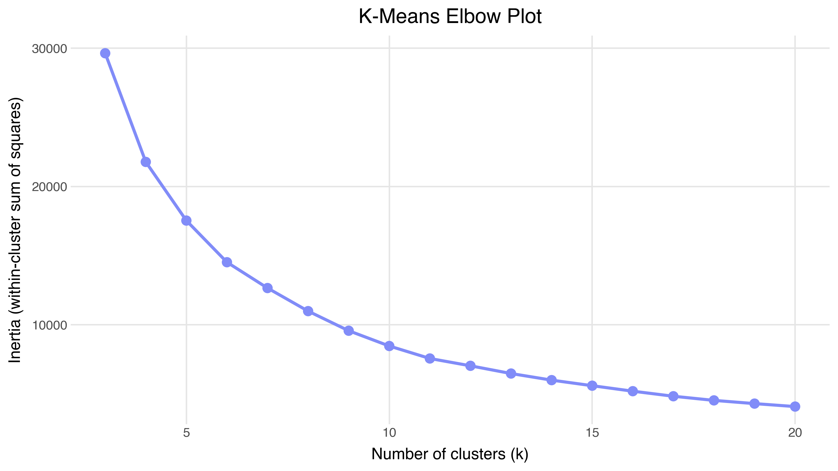
There isn’t a sharp elbow here — the inertia decreases smoothly, which often happens with real data. Embeddings produce continuous structure, not neatly separated blobs.
Silhouette analysis measures how well each point fits its cluster versus the nearest neighboring cluster. A score of 1 means perfect fit; 0 means the point sits on the boundary between clusters; negative means it’s probably in the wrong cluster.
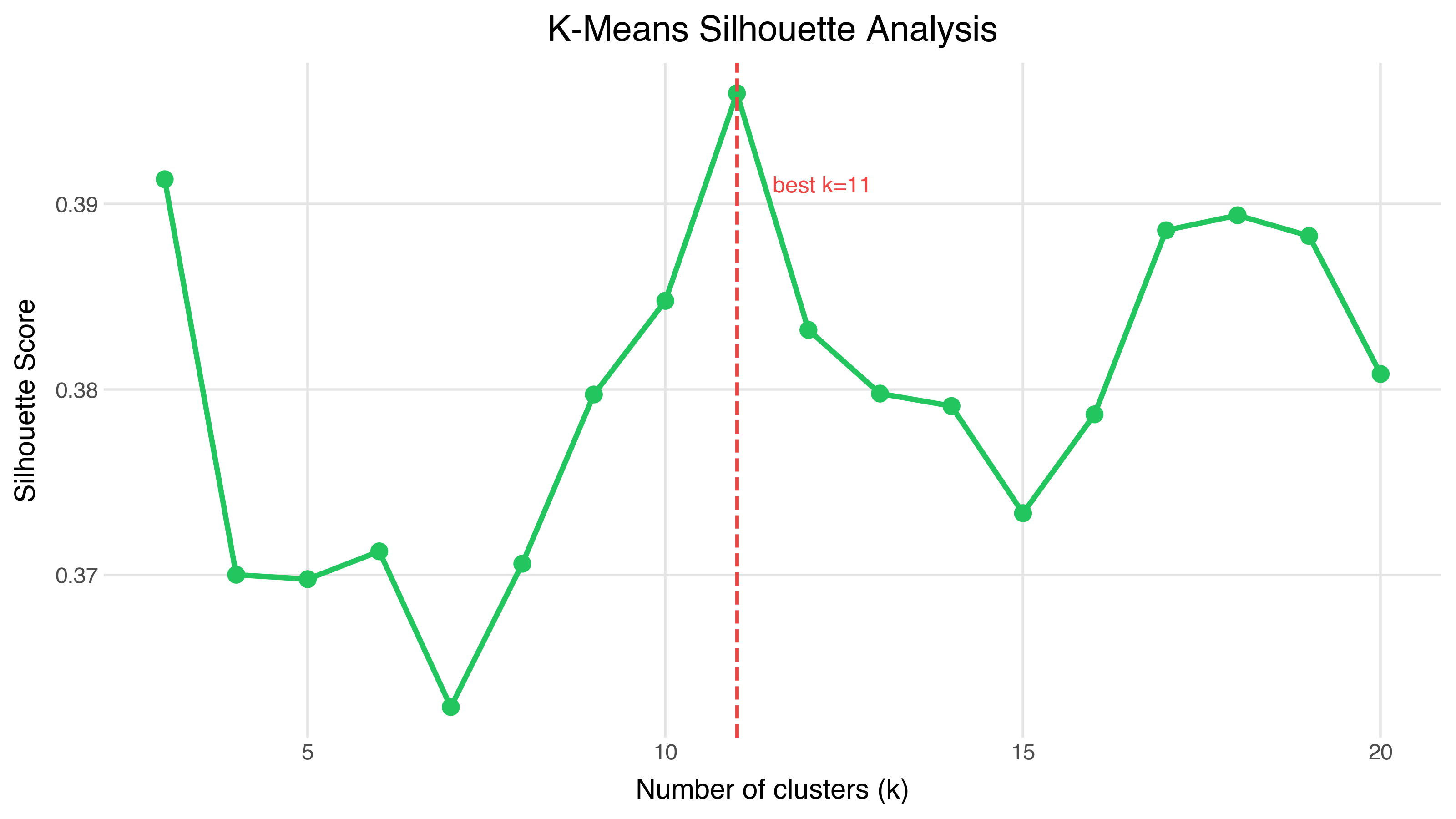
The peak is at k=11, with a silhouette score of 0.396. That’s decent but not spectacular — it’s telling us the data has some cluster structure, but the boundaries aren’t crisp. This is typical for embeddings: semantic space is continuous, not divided into neat compartments.
DBSCAN: “Show Me What’s Dense”
DBSCAN takes a completely different approach. Instead of dividing space into k regions, it says: “a cluster is a dense region separated from other dense regions by sparser space.” Two parameters control this:
- eps: How far apart can two points be and still be neighbors?
- min_samples: How many neighbors does a point need to be “core” (inside a cluster)?
from sklearn.cluster import DBSCAN

db = DBSCAN(eps=0.3, min_samples=10)
labels = db.fit_predict(umap_2d)
DBSCAN doesn’t require choosing k — it discovers the number of clusters from the data. And it naturally handles noise: points that aren’t dense enough to belong to any cluster get labeled as outliers rather than being forced into the nearest group.
With eps=0.3 on our UMAP projections, DBSCAN finds 10 clusters with only 43 noise points (0.4%).
HDBSCAN: “The Right Default”
HDBSCAN (Hierarchical DBSCAN) improves on DBSCAN in two key ways: it handles variable-density clusters (where some clusters are tighter than others) and it has fewer hyperparameters — just min_cluster_size, which has an intuitive meaning: “what’s the smallest group I’d consider a real cluster?”
import hdbscan

hdb = hdbscan.HDBSCAN(min_cluster_size=75, min_samples=10)
labels = hdb.fit_predict(umap_15d)
There’s an important subtlety here. We didn’t run HDBSCAN on the 2D UMAP — we ran it on a 15-dimensional UMAP. Why? Because the 2D projection throws away too much structure. When we ran HDBSCAN on the 2D coordinates, it found only 2 clusters (essentially the sentiment split — positive vs. negative). On the 15D UMAP, it finds 7 meaningful clusters with 512 noise points (5.1%).
This is the recommended approach: use UMAP to reduce dimensionality (but not all the way to 2D), then cluster in that intermediate space, then visualize the clusters on the 2D projection.
Side by Side
Here are all three algorithms, with cluster assignments projected onto the same 2D UMAP:
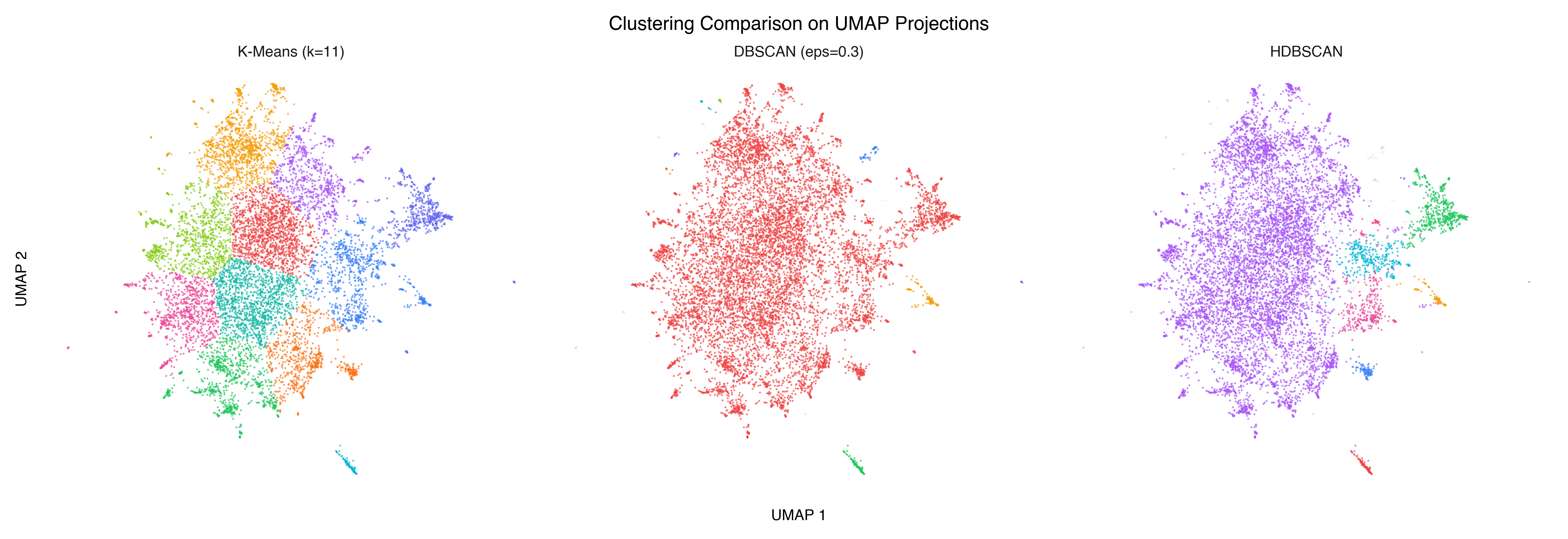
K-means carves the space into equal-ish Voronoi regions — every point gets assigned somewhere, even if the assignment is arbitrary at the boundaries. DBSCAN finds dense cores but can be sensitive to the eps parameter. HDBSCAN produces the most interpretable result: distinct clusters where the data actually clumps, noise where it doesn’t.
What Did HDBSCAN Find?
Let’s zoom in on the HDBSCAN result:
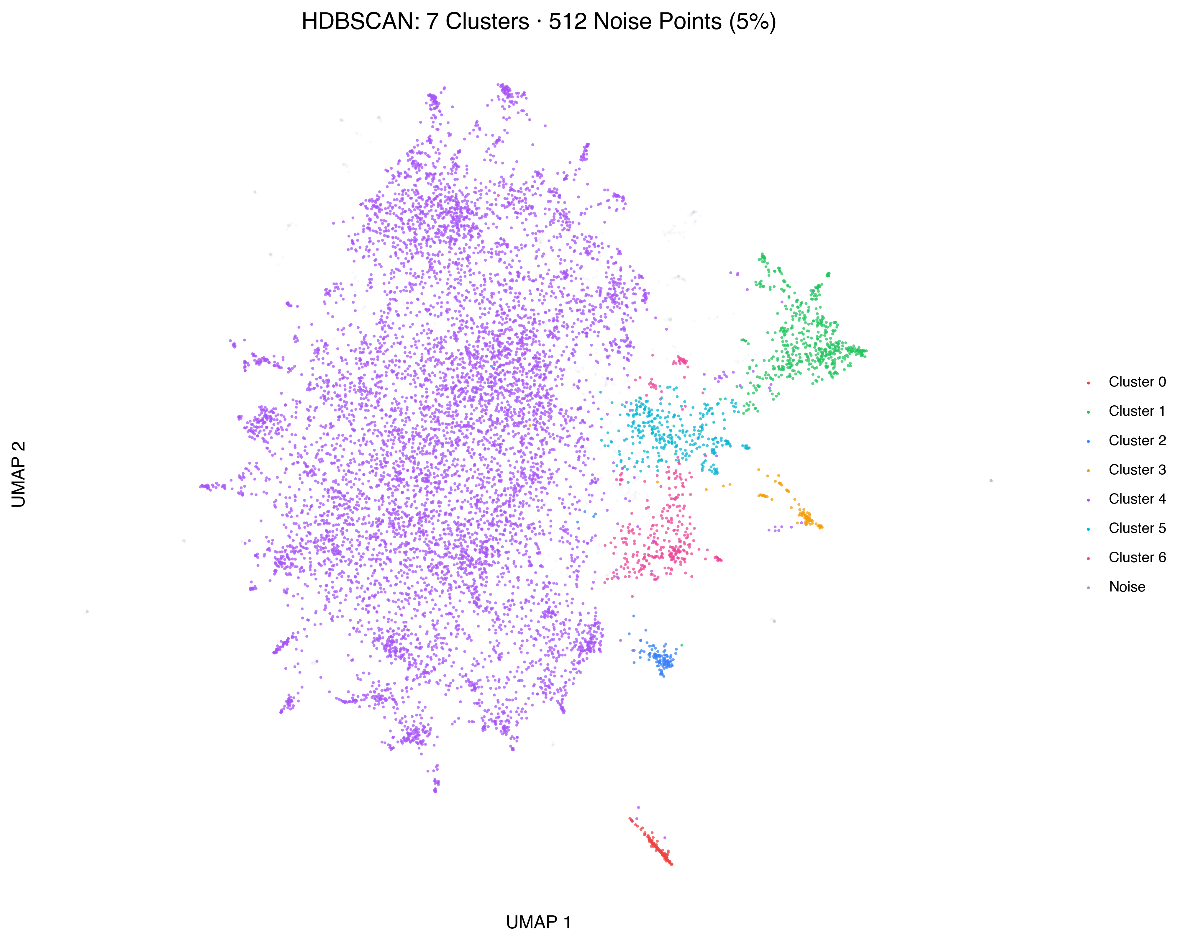
Seven clusters, plus noise. But “Cluster 0” through “Cluster 6” aren’t very informative names. What are these groups actually about?
See It in 3D
Go back to the 3D explorer and switch the coloring to Cluster (HDBSCAN). The cluster assignments we just computed are now available as a third coloring option. Rotate through the data and compare what you see:
- Color by sentiment → two broad regions (positive/negative) with a mixing zone
- Color by rating → a gradient from one pole to the other
- Color by cluster → distinct pockets, mostly within sentiment regions. The clusters subdivide the sentiment landscape by topic.
This is the payoff of the explorer: the same spatial layout tells completely different stories depending on what you color by. Clusters aren’t just about positive vs. negative — they’re about what kind of movie is being reviewed.
Sentiment Purity: The First Sanity Check
Before we try to name the clusters, let’s check whether they correspond to sentiment. Do the clusters separate positive from negative reviews?
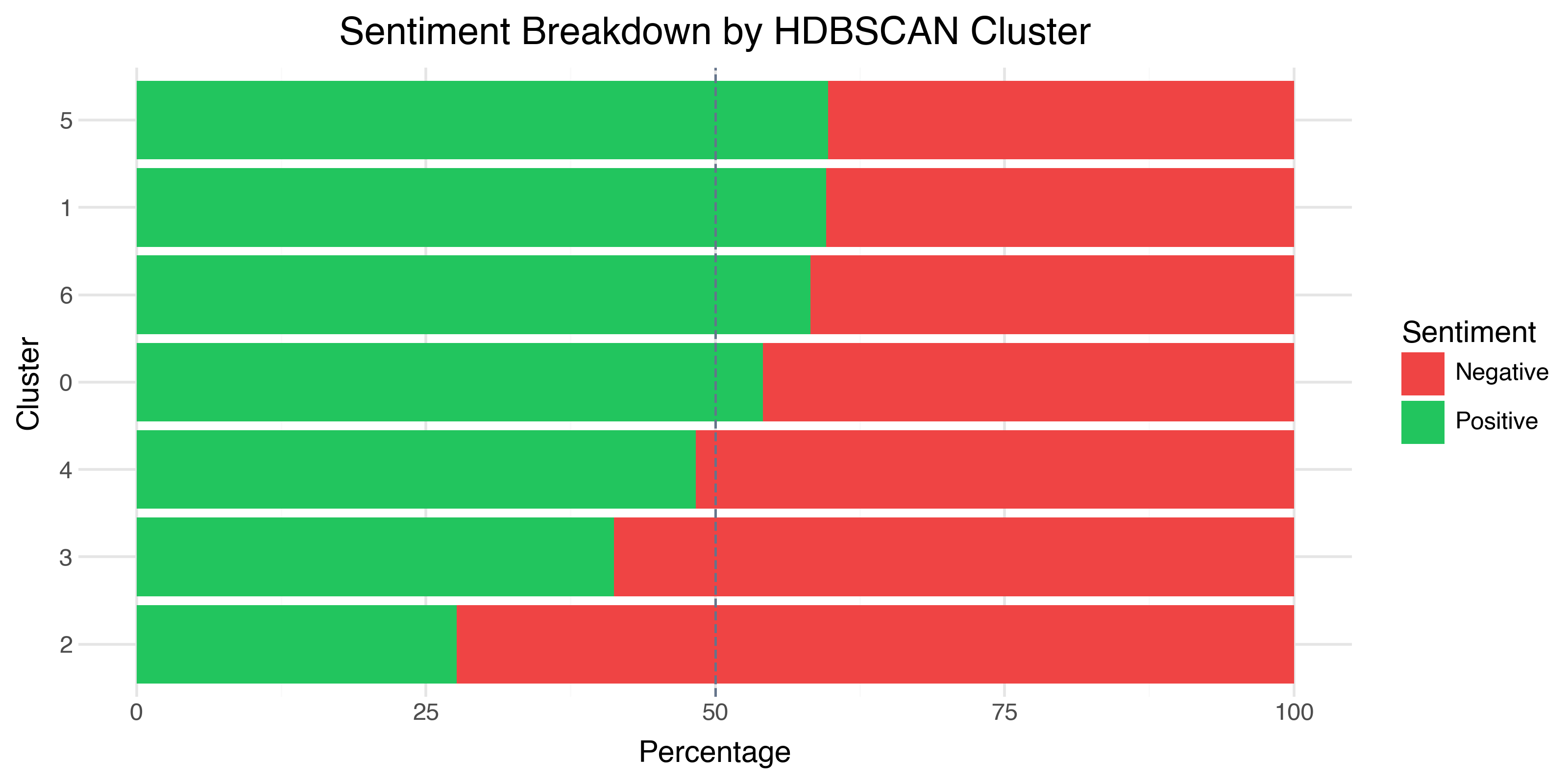
The answer is: mostly not. Most clusters are roughly 50–60% positive — close to the overall dataset balance. This tells us something important: the clusters aren’t about sentiment polarity. They’re about something else — topic, genre, writing style, or cultural context.
The one exception is Cluster 2, which is 72% negative. We’ll see why in a moment.
Naming the Clusters: TF-IDF Keywords
The most direct way to understand a cluster is to find the words that are disproportionately common in it compared to the overall corpus. This is exactly what TF-IDF gives us, with a twist: instead of using raw TF-IDF scores, we subtract the corpus-wide average. The result is a “distinctiveness” score — words that define this cluster versus everything else.
from sklearn.feature_extraction.text import TfidfVectorizer

tfidf = TfidfVectorizer(max_features=5000, stop_words="english")
tfidf_matrix = tfidf.fit_transform(review_texts)

# For each cluster: mean TF-IDF minus corpus mean
cluster_mean = tfidf_matrix[mask].mean(axis=0).A1
corpus_mean = tfidf_matrix.mean(axis=0).A1
distinctiveness = cluster_mean - corpus_mean
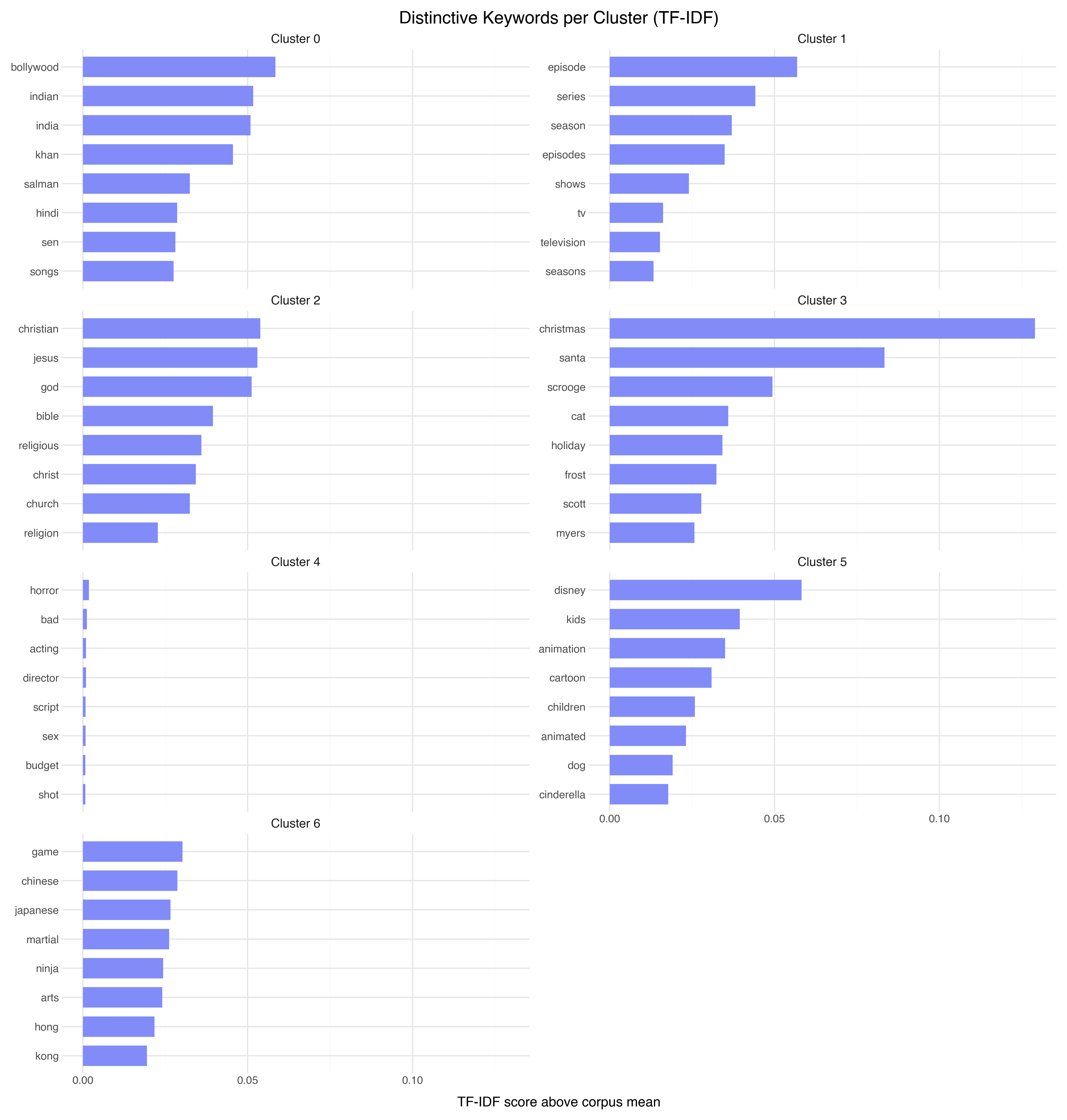
Now the clusters have names:
| Cluster | Size | Keywords | Interpretation |
|---|---|---|---|
| 0 | 146 | bollywood, indian, india, khan | Indian cinema |
| 1 | 517 | episode, series, season, shows | TV series reviews |
| 2 | 112 | christian, jesus, god, bible | Religious films (72% negative!) |
| 3 | 97 | christmas, santa, scrooge, holiday | Holiday movies |
| 4 | 7,953 | horror, bad, acting, director | General reviews (the “everything else” bucket) |
| 5 | 328 | disney, kids, animation, cartoon | Children’s/animated films |
| 6 | 335 | game, chinese, japanese, martial | Martial arts / Asian cinema |
Several things jump out:
The embedding model discovered genre structure that wasn’t in the labels. We gave it raw review text and star ratings — no genre tags, no metadata. Yet it separated Bollywood films, TV shows, animated movies, and martial arts films into distinct regions. The semantic content of reviews contains enough signal to recover genre.
Cluster 2 explains its own sentiment skew. The religious films cluster is 72% negative because many of these reviews are criticizing films for being preachy, inaccurate, or exploitative of religious themes. The embedding grouped them by topic, and the topic happens to correlate with negative sentiment.
Cluster 4 is the “everything else.” At 7,953 points (80% of the data), it’s not really a cluster — it’s the background. Most reviews don’t fall into a niche category. They’re just regular movie reviews. HDBSCAN correctly identifies this as a single dense region rather than splitting it into meaningless subgroups.
Refining Labels with a Cross-Encoder
TF-IDF keyword extraction gives us a strong starting point — we know Cluster 0 is about “bollywood, indian, india, khan.” But keywords are noisy. They tell you what’s frequent, not necessarily what’s defining. A cluster of martial arts reviews might have “film” as a top keyword simply because the word appears in most reviews.
In Post 1, we introduced the bi-encoder / cross-encoder distinction: bi-encoders embed each text independently for fast comparison; cross-encoders take two texts together for more accurate relevance scoring. Here’s where that comes back.
The idea: take the representative reviews from each cluster (the ones nearest to the centroid, which we already computed) and score them against a set of candidate labels using a cross-encoder:
from sentence_transformers import CrossEncoder

reranker = CrossEncoder("cross-encoder/ms-marco-MiniLM-L-6-v2")

candidate_labels = [
    "Bollywood and Indian cinema",
    "TV series and episodic content",
    "Religious and faith-based films",
    "Holiday and Christmas movies",
    "General movie reviews",
    "Children's animation and Disney",
    "Martial arts and Asian cinema",
    "Horror films and slashers",
    "Classic film criticism",
    "Low-budget B-movies",
]

for cluster_id in range(n_clusters):
    # Get the 5 reviews nearest to centroid
    reps = get_representative_texts(cluster_id, n=5)
    combined = " ".join(reps[:3])  # concatenate top 3

    scores = reranker.predict(
        [(combined, label) for label in candidate_labels]
    )
    ranked = sorted(zip(candidate_labels, scores), key=lambda x: -x[1])
    print(f"Cluster {cluster_id}: {ranked[0][0]} ({ranked[0][1]:.3f})")
The cross-encoder doesn’t just check word overlap — it understands that “this Bollywood film lacks the charm of typical Yash Chopra productions” is about Indian cinema even if the word “Indian” never appears. It catches what TF-IDF misses.
For our clusters, the cross-encoder confirmed most of the TF-IDF labels but made a few refinements:
| Cluster | TF-IDF Label | Cross-Encoder Label |
|---|---|---|
| 0 | Indian cinema | Bollywood and Indian cinema |
| 1 | TV series reviews | TV series and episodic content |
| 2 | Religious films | Religious and faith-based films |
| 4 | General reviews | General movie reviews |
| 6 | Martial arts / Asian cinema | Martial arts and Asian cinema |
No surprises here — the TF-IDF keywords were already quite good. Cross-encoders add the most value when the cluster theme is conceptual rather than lexical — when the defining characteristic is a style or attitude that doesn’t reduce to specific keywords.
The Modern Shortcut: LLM-Assisted Labeling
In 2026, there’s a faster way to label clusters. Feed representative documents to an LLM and ask directly:
prompt = """Here are 5 movie reviews from the same cluster.
What do they have in common? Give a 3-5 word label.

Review 1: {rep_1}
Review 2: {rep_2}
Review 3: {rep_3}
Review 4: {rep_4}
Review 5: {rep_5}
"""
For our clusters, an LLM produced:
| Cluster | TF-IDF | LLM Label |
|---|---|---|
| 0 | bollywood, indian, india, khan | “Bollywood fan reviews” |
| 1 | episode, series, season, shows | “TV series binge reviews” |
| 2 | christian, jesus, god, bible | “Religious film criticism” |
| 3 | christmas, santa, scrooge, holiday | “Holiday movie nostalgia” |
| 4 | horror, bad, acting, director | “Mixed general opinions” |
| 5 | disney, kids, animation, cartoon | “Family animation reviews” |
| 6 | game, chinese, japanese, martial | “Asian action cinema” |
The LLM labels capture tone (“nostalgia,” “criticism,” “binge”) that neither TF-IDF nor cross-encoders can easily surface. This is the practical approach most developers will reach for in production — and it works remarkably well as long as you verify the labels against the data rather than trusting them blindly.
The three-method pipeline is: TF-IDF gives you the keywords → cross-encoder refines ambiguous cases → LLM produces human-readable labels. In practice, you might skip the middle step if your clusters have clear keyword signatures, but for subtle or overlapping clusters, cross-encoder scoring catches what bag-of-words methods miss.
A Second Lens: NMF Topic Modeling
Clustering works in the spatial domain — it groups points that are near each other in embedding space. But there’s a complementary approach: topic models work directly on the word distributions, decomposing the corpus into overlapping topics without reference to the embedding coordinates at all.
NMF (Non-negative Matrix Factorization) factors the document-term matrix into two matrices: one mapping documents to topics, and one mapping topics to words. The non-negativity constraint means each topic is an additive combination of words, which produces interpretable results.
from sklearn.decomposition import NMF

nmf = NMF(n_components=7, random_state=42, max_iter=500)
W = nmf.fit_transform(tfidf_matrix)  # document-topic weights
H = nmf.components_                   # topic-word weights
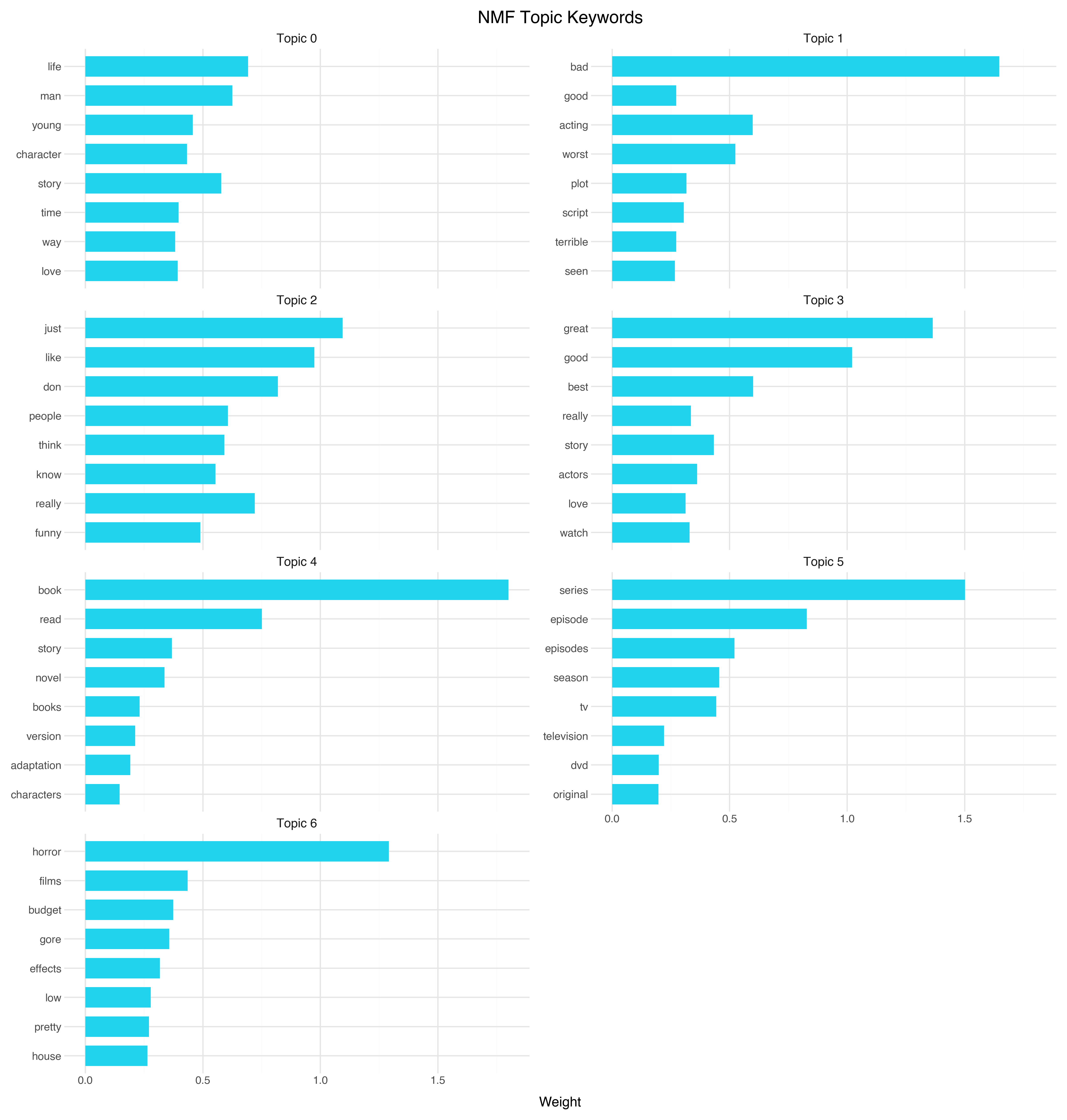
The NMF topics are:
| Topic | Keywords | Interpretation |
|---|---|---|
| 0 | life, man, story, young, character | Character-driven drama |
| 1 | bad, acting, worst, plot, script | Negative reviews (the “this movie is terrible” topic) |
| 2 | just, like, don, really, people | Conversational/casual reviews |
| 3 | great, good, best, story, actors | Positive reviews (the “this movie is excellent” topic) |
| 4 | book, read, story, novel | Book adaptations |
| 5 | series, episode, episodes, season | TV series |
| 6 | horror, films, budget, gore | Horror films |
Interesting — NMF and HDBSCAN tell overlapping but distinct stories. Both found TV series (Cluster 1 / Topic 5) and both found a horror-adjacent group. But NMF discovered a sentiment dimension (Topics 1 and 3 are essentially “bad movies” and “good movies”), while HDBSCAN found cultural dimensions (Bollywood, martial arts, religious films) that NMF missed entirely.
Do They Align?
We can measure the overlap by computing, for each cluster, the average NMF topic weight:
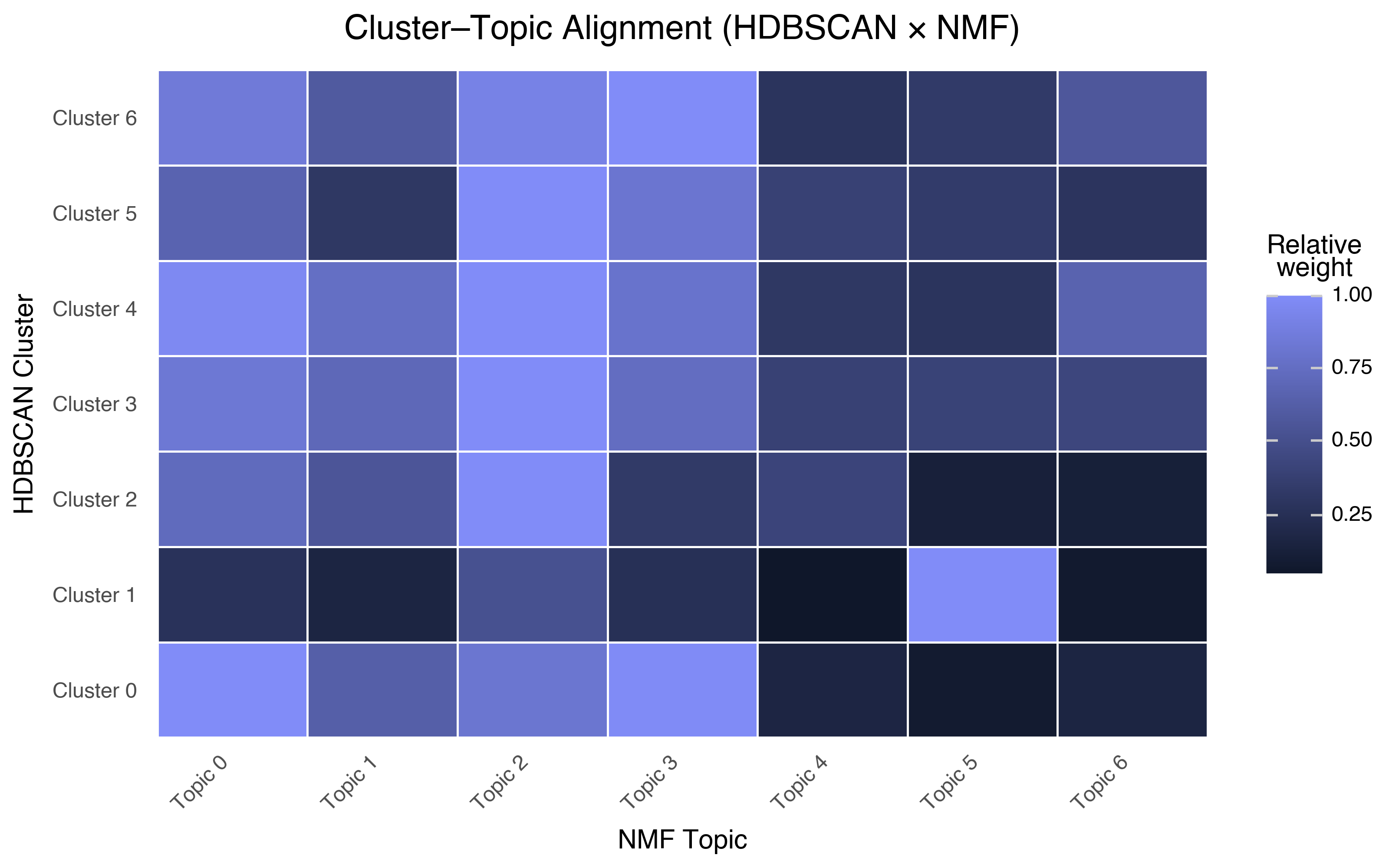
Each row is an HDBSCAN cluster; each column is an NMF topic. Bright cells mean a cluster aligns strongly with a topic. A few observations:
Cluster 1 (TV series) maps cleanly to Topic 5 (TV series). Both methods independently found the same structure. When two methods agree, you can be more confident the pattern is real.
Cluster 4 (the “everything else”) has moderate weight across many topics. This makes sense — it’s the undifferentiated mass of general reviews, and it contains a bit of everything.
The niche clusters (Bollywood, religious, martial arts) don’t map to any single NMF topic. These clusters are defined by cultural vocabulary that NMF distributes across multiple topics. Spatial clustering in embedding space found structure that word-frequency decomposition couldn’t.
This is the payoff of using multiple methods. Each one captures different aspects of the data’s structure. Together, they give you a richer understanding than either alone.
When Clusters Are Artifacts
Not every clump you see is real. Here are some warning signs:
Clusters that disappear under different parameters. If you run HDBSCAN with min_cluster_size=75 and get 7 clusters, but min_cluster_size=50 gives you 32 clusters (with 46% noise), that middle ground is fragile. The 7-cluster solution is more stable.
Clusters that appear only in the 2D projection. We saw this: HDBSCAN on the 2D UMAP found only 2 clusters. The other 5 clusters are real in the higher-dimensional space but invisible when projected flat. Always be suspicious of clusters you can only see in 2D.
Clusters with no semantic coherence. If you extract keywords and get nothing distinctive — just generic words — the cluster is probably an artifact of the spatial arrangement, not a meaningful group.
The biggest cluster. When one cluster contains 80% of your data, it’s not really a “cluster” — it’s the background. The interesting structure is in the smaller groups and the noise points at the edges.
Key Takeaways
K-means, DBSCAN, and HDBSCAN have different philosophies. K-means partitions, DBSCAN finds density, HDBSCAN handles variable density. For exploratory work, HDBSCAN on a moderate-dimensional UMAP is usually the best starting point.
Don’t cluster on your 2D visualization. Use 10–15 UMAP dimensions for clustering, then project back to 2D for display. The 2D projection throws away too much structure.
Three labeling methods, each with a strength. TF-IDF keywords tell you what’s frequent, cross-encoders tell you what’s relevant, and LLMs tell you what’s meaningful. Use them in combination for the most robust cluster labels.
NMF topic models are a complementary lens. They decompose word distributions without reference to spatial structure. When topics and clusters agree, you can be confident. When they disagree, the difference is informative.
The embedding model discovered genre without genre labels. From raw review text alone, the semantic space separated Bollywood, TV series, animation, religious films, and martial arts into distinct regions. This is a strong validation of the embedding quality.
Most of the data doesn’t cluster. And that’s fine. The 80% of reviews in the “general” cluster are genuinely generic — regular movie opinions that don’t have enough niche vocabulary to separate. The interesting structure is at the edges.
References
- Campello, Moulavi & Sander (2013) — “Density-Based Clustering Based on Hierarchical Density Estimates” — The HDBSCAN paper
- Ester et al. (1996) — “A Density-Based Algorithm for Discovering Clusters in Large Spatial Databases with Noise” — The original DBSCAN paper
- Lee & Seung (1999) — “Learning the parts of objects by non-negative matrix factorization” — NMF for parts-based decomposition
- Reimers & Gurevych (2019) — “Sentence-BERT” — Cross-encoders for pairwise relevance scoring
- HDBSCAN documentation — Excellent guide to parameter selection