Feature Engineering — Beyond the Embedding

We’ve come a long way with just embeddings. From 768-dimensional vectors, we’ve built statistics, projections, an interactive 3D explorer, and meaningful clusters — all from a single representation of text meaning.

But embeddings are a compression. They capture what the model was trained to encode — semantic similarity, topical relatedness, sentiment — and discard everything else. What about the information that isn’t in the text?

This post is about going beyond the embedding: extracting structured features from the text and discovering what they reveal that the embedding alone can’t see.

Features as Lenses

The most powerful idea in this post isn’t a technique — it’s a strategy. Instead of concatenating features into the embedding and re-running UMAP, use features as lenses: color the same spatial layout by different variables and see what patterns emerge.

The UMAP projection stays fixed — it captures the semantic structure of the reviews. But what we see changes completely depending on what we color by.

Review Length

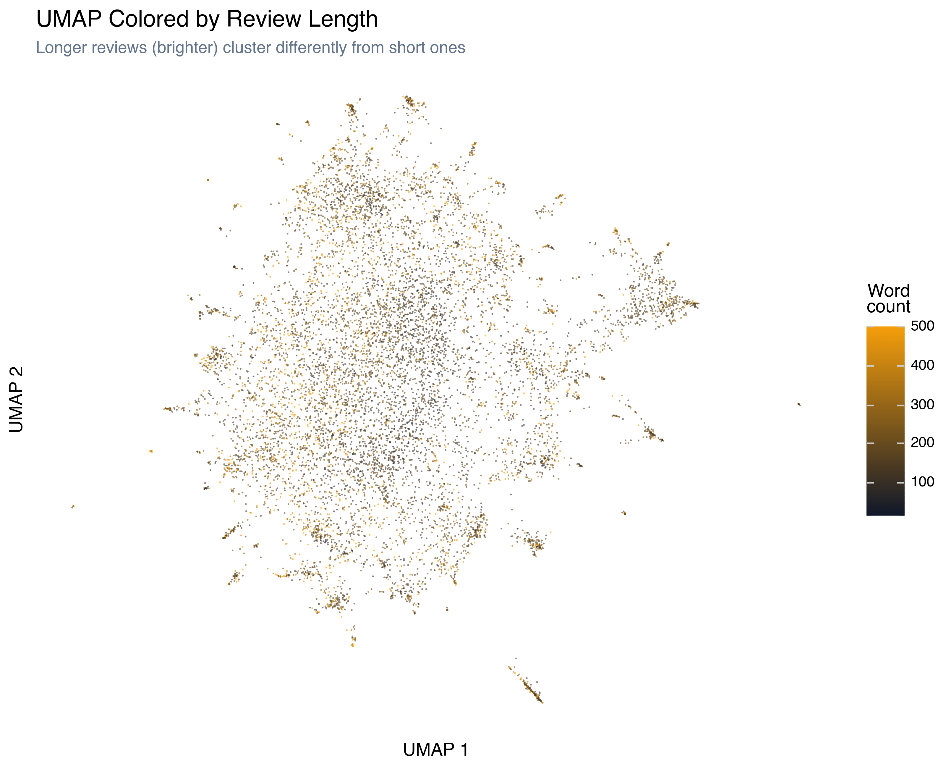
Longer reviews (brighter) don’t cluster randomly — they tend to occupy specific regions. The dense core of the projection has a mix of lengths, but the periphery shows pockets of very short reviews and pockets of very long ones. Short reviews tend to be more extreme (strong love or strong hate in few words), while long reviews are often more analytical.

Vocabulary Richness

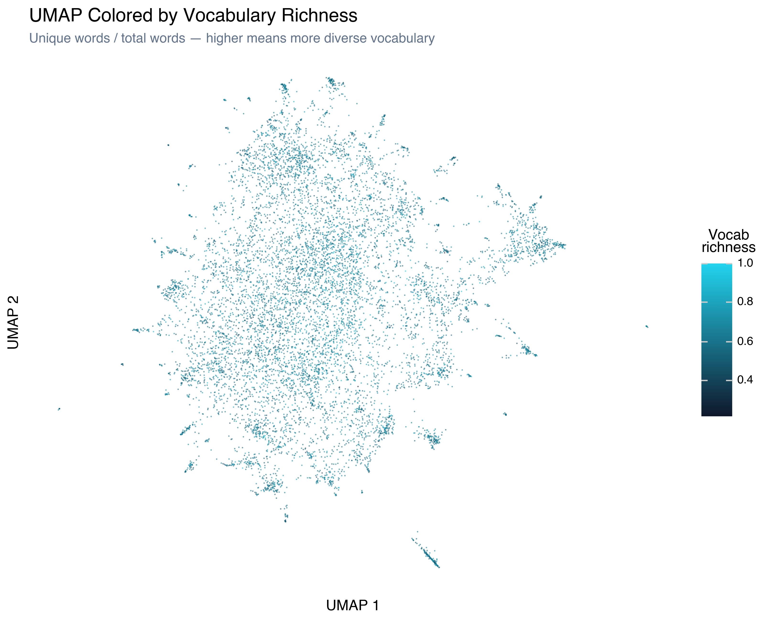
Vocabulary richness — unique words divided by total words — is a crude proxy for writing sophistication. High-richness reviews (brighter) tend to cluster together, especially in regions that correspond to more literary or critical writing. Low-richness reviews often contain repetitive language (“bad bad bad” or “great great movie”).

Genre Keywords

This is the most revealing lens. We detected genre-related keywords in each review (horror, comedy, romance, sci-fi, war, animation, documentary, thriller) and colored by the dominant genre:

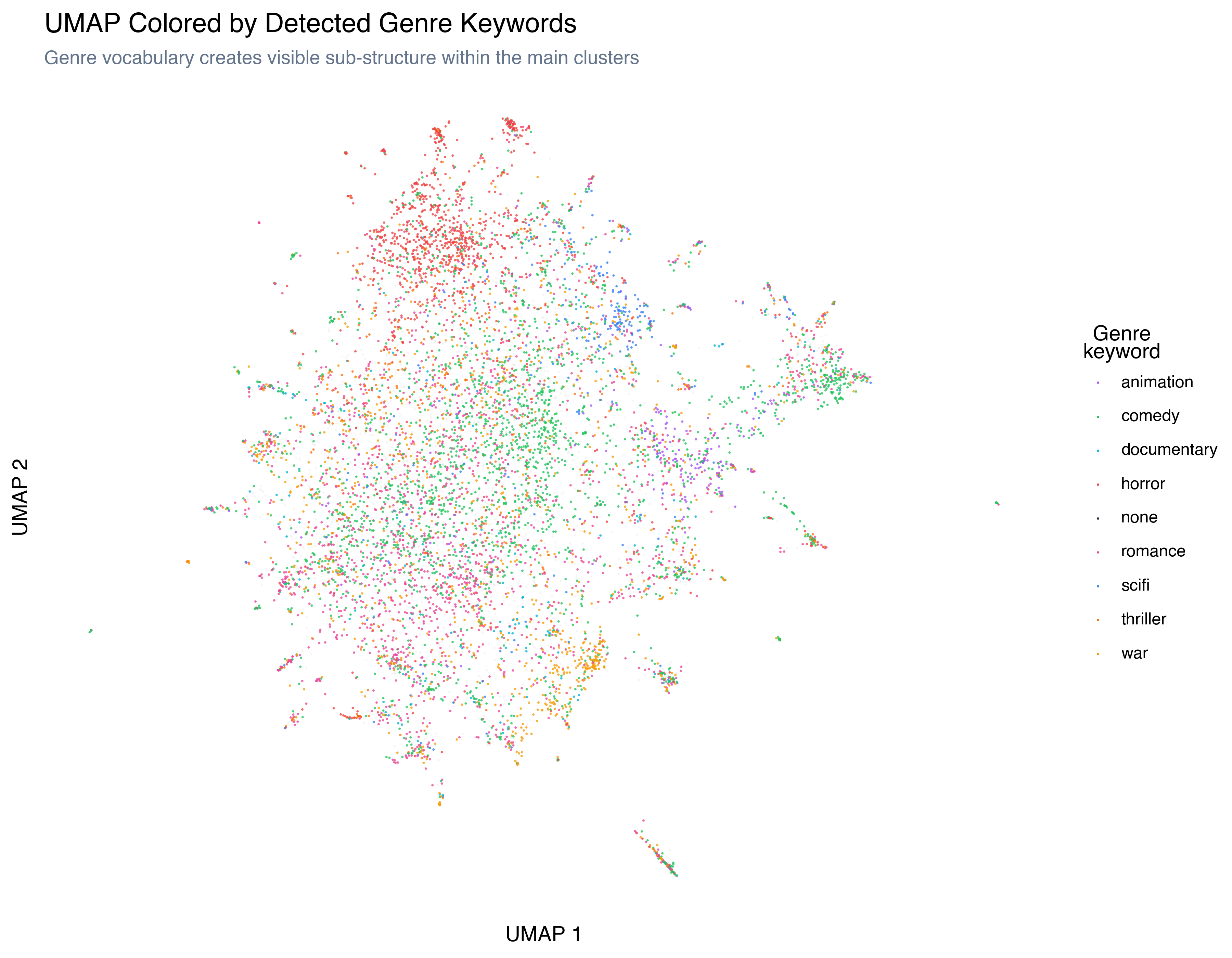
Genre vocabulary creates visible sub-structure within the main clusters. The horror reviews (red) occupy a distinct region; comedy (green) and romance (pink) overlap significantly (romantic comedies are a thing); animation reviews (purple) form a tight cluster matching what HDBSCAN found in Post 5.

This is a key insight: the embedding model captured genre structure implicitly, just from the review text, even though it was never given genre labels. The genre keywords we extracted merely name a structure that was already present in the embedding space.

The Concatenation Problem

The obvious next question: if structured features carry useful signal, why not just add them to the embedding? Concatenate the 768-dimensional embedding vector with 13 structured features, run UMAP on the combined 781 dimensions, and get a “richer” projection.

Here’s what happens:

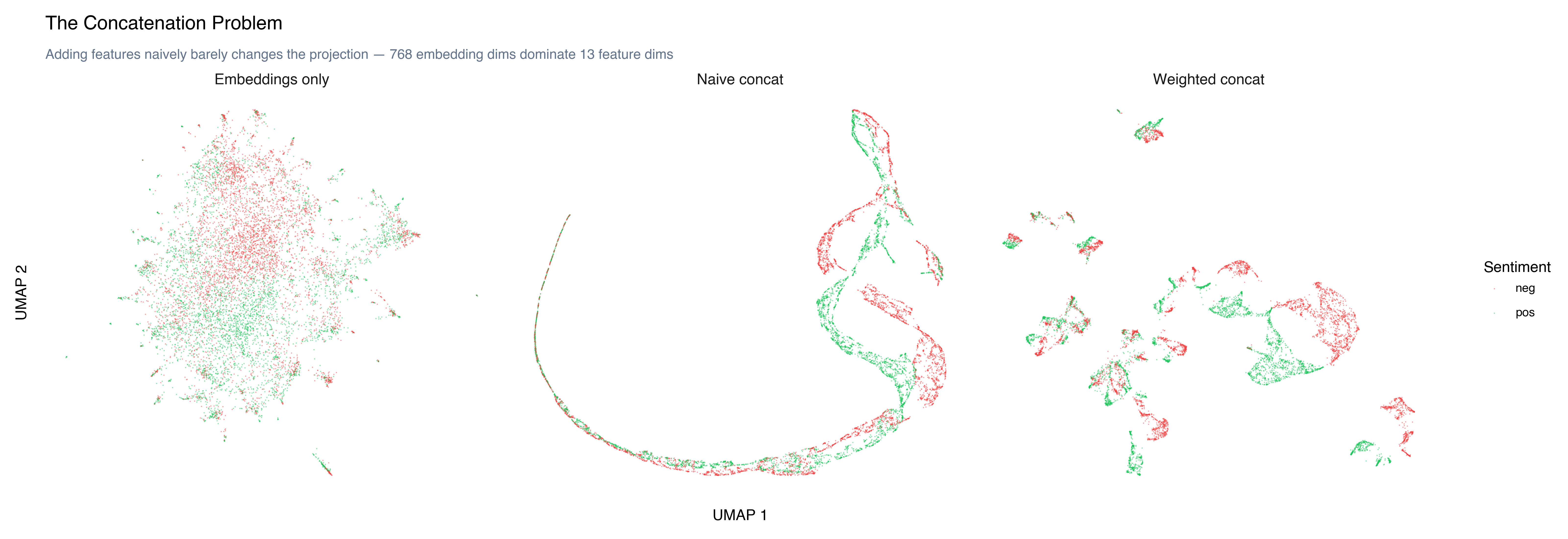
The naive concatenation (center) looks radically different from the embeddings-only projection (left) — but not in a good way. Despite having only 13 extra features versus 768 embedding dimensions, the raw features dominate. Why? Because embedding dimensions typically have values between -1 and 1, while word_count ranges from 0 to 500+ and rating from 1 to 10. In Euclidean distance, a single feature with large magnitude contributes more than hundreds of features with small magnitude. The result is a projection driven primarily by review length and rating rather than semantic content — the swirly, elongated shape is the UMAP trying to organize points by a few high-variance scalars.

The weighted version (right) makes things worse by amplifying the structured features even further (7.7x), fragmenting the semantic structure into disconnected islands organized by feature values rather than meaning.

The lesson: there’s no “just right.” Either the structured features are too small to affect the projection (pointless), or they’re large enough to distort it (harmful). Concatenation is the wrong approach.

Why Concatenation Is Usually Wrong

We just saw the scale problem in action: a handful of large-valued features can overpower hundreds of small-valued embedding dimensions. But the deeper issue isn’t just scale — it’s semantic mismatch:

• Embedding dimensions are dense and continuous. Every dimension carries a small piece of the overall meaning. No single dimension is interpretable.
• Structured features are sparse and interpretable. A genre_horror flag is either 0 or 1, and you know exactly what it means.

Mixing these two types of features into a single vector is like adding paragraph text and checkboxes into the same search index. The mathematically correct combination depends on what question you’re asking.

Better approaches:

1. Use features as lenses (what we did above) — keep the embedding space intact, use structured features to color/filter/annotate.

2. Separate projections — run UMAP on the embedding and separately on the structured features, then compare the two layouts.

3. Use features for evaluation — cluster on embeddings, then use structured features to validate the clusters (as we did with sentiment in Post 5).

4. Multi-view learning — train a model that learns a shared low-dimensional space respecting both feature types. This is the “right” solution but requires training infrastructure.

For exploratory analysis, option 1 almost always wins. It’s fast, it’s interpretable, and it doesn’t risk corrupting the embedding structure with noisy features.

Try It Yourself: The Feature Mixing Board

What if you could control the concatenation weights and see the resulting UMAP instantly? Below, we’ve pre-computed a genuine UMAP projection for every combination of slider weights:

• Meaning: the sentence-transformer embedding (768 dimensions)
• Genre: eight keyword-detection features (horror, comedy, romance, sci-fi, war, animation, documentary, thriller)
• Style: writing characteristics (word count, vocabulary richness, sentence length, exclamation rate)

Each feature group is normalized independently (StandardScaler) and scaled by 1/√dims so that each group contributes equally at equal weight regardless of its dimensionality. Every layout you see is a real UMAP — not an interpolation or approximation. Each slider combination triggers a genuinely different dimensionality reduction.

A few things to try:

1. Start with just Meaning (the default). This is the familiar semantic UMAP we’ve been exploring all series.

2. Slide Genre up to 100, Meaning down to 0. Watch the topology completely change. With only 8 binary features, UMAP creates tight, separated islands — one per genre combination. Sentiment coloring loses all spatial coherence (genre and sentiment are nearly independent).

3. Now try Style alone. Another dramatic restructuring: reviews organized by how they’re written rather than what they’re about. Switch to rating coloring — do you see a relationship between writing style and rating?

4. Set Meaning to 75, Genre to 25. Compare to pure Meaning — the topology is recognizably similar but subtly different. The genre signal nudges some clusters apart and pulls others together. This is what concatenation actually does when the weights are balanced by normalization.

5. Try all three at equal weight (25/50/25 or similar). The UMAP has to find structure that respects all three notions of similarity simultaneously. Clusters that are semantically tight, genre-consistent, and stylistically similar survive; others fragment.

Notice something unsettling? As you slide between nearby weight combinations, the layout doesn’t morph smoothly — it jumps. Move a slider one tick and the entire cloud reorganizes. Move it again in the same direction and the reorganization goes in a completely different direction. The sliders feel linear, but the output is anything but.

This isn’t a bug. UMAP is a stochastic, nonlinear optimization that finds a 2D layout preserving local neighbor structure — not the layout. Small weight changes cause different points to become each other’s nearest neighbors, which cascades through the entire graph. UMAP’s gradient descent converges to a different local minimum. There’s no constraint that similar inputs should produce similar outputs.

This is arguably the most important thing the mixing board reveals. We’ve been treating UMAP projections as maps throughout this series — spatial arrangements that mean something. And they do, locally: nearby points really are similar. But the global arrangement (which cluster is on the left, whether two groups are adjacent or separated) is arbitrary. Two runs of UMAP on the same data with different random seeds would give different global layouts. Changing the feature weights is even more dramatic.

The practical takeaway: with proper normalization and equal-variance scaling, concatenation does produce meaningful results — the scale mismatch we saw earlier was the real problem, not the approach itself. But trust the clusters, not their positions.

Feature Distributions by Cluster

One last lens: how do the structured features distribute across HDBSCAN clusters? If different clusters have different feature profiles, that tells us the clusters are capturing something beyond just topic.

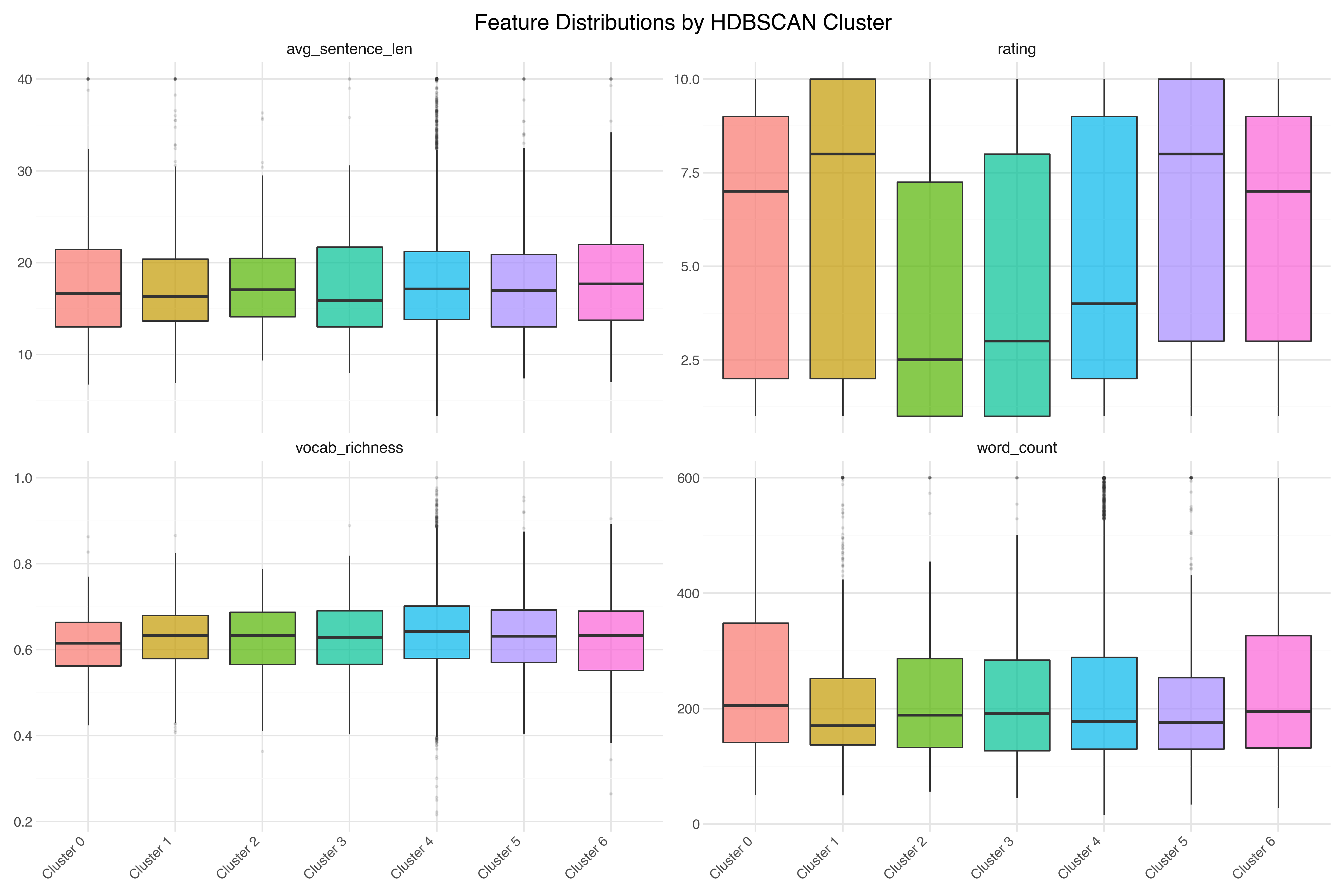
The distributions reveal that:

• Review length varies by cluster. TV series reviews (Cluster 1) tend to be longer — people have more to say about a whole season. Christmas movie reviews (Cluster 3) tend to be shorter.

• Vocabulary richness is relatively stable across clusters, but the animation cluster (Cluster 5) has slightly lower richness — simpler language, matching the target audience.

• Rating distributions differ. The religious films cluster (Cluster 2) skews heavily negative. The martial arts cluster (Cluster 6) has a wider spread.

Each of these observations would take minutes of statistical testing to confirm formally. With the right visualization, you can see them in seconds.

Key Takeaways

1. Features as lenses, not inputs. Don’t concatenate structured features into your embedding. Use them to color and filter your existing visualizations. The insight comes from seeing how different features correlate with the spatial structure.

2. The concatenation problem is real. A few high-magnitude features (word count, rating) can distort 768 embedding dimensions, and weighting makes it worse. Scale mismatch and semantic mismatch make naive combination unreliable in both directions.

3. Proper normalization rescues concatenation. With per-group StandardScaler and 1/√dims variance equalization, weighted concatenation produces genuine, interpretable results — the feature mixing board proves it.

4. The embedding model knew more than we asked. Genre, writing style, review length, cultural context — all were encoded in the 768 dimensions. We just needed the right lenses to see them.

5. UMAP projections are local, not global. The mixing board reveals that similar inputs can produce very different global layouts. Trust the clusters, not their positions on the page.

References

• McInnes, Healy & Melville (2018) — “UMAP: Uniform Manifold Approximation and Projection” — The algorithm behind the projections
• McInnes et al. (2017) — “hdbscan: Hierarchical density based clustering” — HDBSCAN reference

Previous: Making Sense of Clusters

Next: Graph Analysis — When Connections Tell the Story