What Embeddings Actually Are
I learned about word2vec the way most interesting things arrive in a career: someone smarter than me was excited about it and their excitement was contagious.
Vectors at Hulu
In 2013, I was a software engineer at Hulu, building data pipelines for the ad platform. Two colleagues — Dr. Hang Li (now at Meta) and Dr. Kevin Lin (now at Waymo) — were excited about a paper from Google. Tomáš Mikolov and his team had published a method for learning vector representations of words that was fast, simple, and produced results that felt almost magical.
The core idea: take a huge pile of text, and learn a vector — a list of numbers — for each word, such that words used in similar contexts end up as nearby points in the same geometric space. The method was called word2vec.
What made it magical was what the geometry captured. The most famous example:
king - man + woman ≈ queen
This wasn’t a lookup table or a hand-coded rule. The model had learned, purely from patterns of word co-occurrence, that the direction from “man” to “woman” was the same as the direction from “king” to “queen.” Gender, royalty, tense, geography — these abstract relationships emerged as directions in space.
I experimented with it, played with the analogies, and felt the same kind of wonder I’d felt years earlier watching a neural net learn. But at the time, I was deep in pipeline architecture and didn’t push further.
It was only later that I’d understand just how foundational this idea was.
The Geometry of Words
Let’s make this concrete. A word2vec model assigns every word a vector — say, 300 numbers. You can load a pre-trained model and start asking questions:
import gensim.downloader as api

# Load a pre-trained word2vec model (trained on Google News, 3 billion words)
model = api.load("word2vec-google-news-300")

# The classic analogy
result = model.most_similar(positive=["king", "woman"], negative=["man"], topn=3)
for word, score in result:
    print(f"  {word:15s} {score:.3f}")
  queen           0.712
  monarch         0.619
  princess        0.590
The model has never been told what “king” or “queen” means. It’s never seen a definition. It learned these relationships entirely from which words appear near which other words in billions of sentences.
Here’s the intuition: in English text, “king” and “queen” appear in similar contexts (ruling, crowns, thrones), so they end up near each other. But “king” also appears in contexts similar to “man” (he, his, himself), and “queen” in contexts similar to “woman” (she, her, herself). The model resolves both patterns simultaneously by placing these words in a space where the direction from male to female is consistent across the royalty axis.
This works for all kinds of relationships:
# Geography
model.most_similar(positive=["Paris", "Germany"], negative=["France"], topn=1)
# → [('Berlin', 0.747)]

# Verb tense
model.most_similar(positive=["walking", "swam"], negative=["walked"], topn=1)
# → [('swimming', 0.764)]

# What's most similar to a word?
model.most_similar("python", topn=5)
# → [('pythons', 0.70), ('snake', 0.65), ('Burmese_python', 0.63), ...]
Each of these queries is just arithmetic on vectors. “Paris minus France plus Germany” is literally subtracting one list of 300 numbers from another and adding a third. The fact that this arithmetic lands on “Berlin” is a consequence of the geometric structure the model learned.
Finding Relationships in Netflix’s Vocabulary
Years later, at Netflix, I was working on knowledge management systems — tools to help people find and share information across a large engineering organization. We had a growing corpus of internal documents, mostly research memos.
I trained a word2vec model on these internal documents. The corpus was small by internet standards — nothing like the billions of words Google had used — but I wanted to see whether the geometric structure would appear even in a specialized, limited vocabulary.
It did.
The model learned relationships between team names, product names, and technical concepts that mirrored the company’s actual organizational structure. Analogies between systems worked. Nearest-neighbor queries surfaced documents that were semantically related in ways that keyword search would never find.
I also found that even with just this internal corpus, the classic analogy patterns replicated — the “king/queen → man/woman” style relationships appeared between our own domain-specific terms. The embedding space had captured real semantic structure in the company’s vocabulary, and it had done so purely from patterns in how people wrote.
From Words to Documents
Word2vec gives you a vector for each word. But what about a whole sentence? A paragraph? A document?
The simplest approach is averaging: take the word vectors for every word in a document and compute their mean. This works surprisingly well for many applications — it’s fast and captures the general “topic” of the text. But it’s lossy. “The dog bit the man” and “The man bit the dog” produce the same average, because order is discarded.
The modern solution is embedding models — transformer networks (the same architecture behind GPT and BERT) fine-tuned specifically to produce good sentence- and document-level embeddings, where semantically similar texts produce similar vectors.
The landscape of embedding models has evolved quickly. A few landmarks:
- Sentence-BERT (2019) — The original fine-tuned BERT approach for sentence embeddings. The sentence-transformers library grew from this work and remains the standard open-source toolkit.
- BGE (BAAI, 2023) — Models like
bge-large-en-v1.5significantly outperform the earlier sentence-transformers defaults on retrieval benchmarks. - OpenAI embeddings (2024) —
text-embedding-3-smallandtext-embedding-3-largeoffer strong quality via API, and are what many developers encounter first in practice. - Qwen3-Embedding (2025) — The latest generation of open-source models from Alibaba, ranging from 0.6B to 8B parameters. The 8B version currently tops the MTEB leaderboard.
For this series, we’ll use all-mpnet-base-v2 — an older (2021) but well-understood model that produces 768-dimensional embeddings. It’s small, fast, runs on CPU, and is more than sufficient for the concepts we’re exploring. The techniques and workflows in this series transfer to any embedding model — if you swap in BGE or Qwen3-Embedding, the analysis pipeline stays the same. Only the quality of the embeddings improves.
from sentence_transformers import SentenceTransformer

# The sentence-transformers library loads most open-source embedding models.
# We use all-mpnet-base-v2 for speed and simplicity;
# bge-large-en-v1.5 or Qwen3-Embedding-0.6B would also work here.
model = SentenceTransformer("all-mpnet-base-v2")

sentences = [
    "The movie was absolutely brilliant, a masterpiece of storytelling.",
    "This film was terrible, a complete waste of time.",
    "An incredible cinematic experience with stunning performances.",
    "I'd like to order a pepperoni pizza with extra cheese.",
]

embeddings = model.encode(sentences, normalize_embeddings=True)
print(f"Shape: {embeddings.shape}")  # (4, 768)
Each sentence is now a point in 768-dimensional space. The positive movie reviews should be near each other, the negative review nearby but in a different region, and the pizza order should be far from all of them.
But how do we measure “near” and “far” in 768 dimensions?
Cosine Similarity: Measuring Semantic Distance
The standard way to compare embedding vectors is cosine similarity: the cosine of the angle between them. Two vectors pointing in the same direction have a cosine similarity of 1. Perpendicular vectors score 0. Opposite directions score -1.
Why cosine and not regular Euclidean distance? Because we care about the direction a vector points, not its magnitude. A long review and a short review about the same topic should be similar, even if one vector has larger values simply because there was more text.
(When we normalize our embeddings to unit length — which we did above — cosine similarity reduces to the dot product. This is a nice computational shortcut.)
import numpy as np

# Cosine similarity between all pairs
similarity_matrix = embeddings @ embeddings.T

labels = ["Positive review 1", "Negative review", "Positive review 2", "Pizza order"]

for i in range(len(sentences)):
    for j in range(i + 1, len(sentences)):
        print(f"  {labels[i]:20s} ↔ {labels[j]:20s}  {similarity_matrix[i,j]:.3f}")
  Positive review 1    ↔ Negative review       0.527
  Positive review 1    ↔ Positive review 2      0.813
  Positive review 1    ↔ Pizza order             0.033
  Negative review      ↔ Positive review 2      0.379
  Negative review      ↔ Pizza order             0.009
  Positive review 2    ↔ Pizza order             0.029
The two positive reviews are highly similar (0.81). The negative review is moderately similar to the positive ones (they’re all about movies, after all). And the pizza order is essentially orthogonal to everything — cosine similarity near zero.
This is what embeddings give you: a principled, numerical way to ask “how similar are these two pieces of text?” — and get an answer that aligns with human intuition.
The Hello World: Embedding My Own Blog Posts
Let’s scale this up slightly. I embedded all 43 posts from this blog using the same all-mpnet-base-v2 model. Each post becomes a single 768-dimensional vector based on its title, description, and first 500 words.
The question: does the embedding space capture the series structure? Posts in the same series cover related topics — will they end up near each other?
import json
import numpy as np

# Load pre-computed embeddings
data = np.load("data/blog_embeddings.npz", allow_pickle=True)
embeddings = data["embeddings"]   # shape: (43, 768)
titles = data["titles"]
series = data["series"]

# Cosine similarity = dot product for unit vectors
similarity = embeddings @ embeddings.T

print(f"Posts: {embeddings.shape[0]}")
print(f"Series: {sorted(set(s for s in series if s))}")
Posts: 43
Series: ['Entity Detection', 'HyperLogLog',
         'Hulu Data Platform', 'Mergeable Operations', 'Neural Nets from Scratch',
         'NYC Taxis and Tipping', 'Python for Fixed-Income Risk Analysis',
         'Tries', 'Writing Agent Skills']
Here’s the similarity matrix, with posts sorted by series. Each cell shows the cosine similarity between two posts — brighter means more similar:
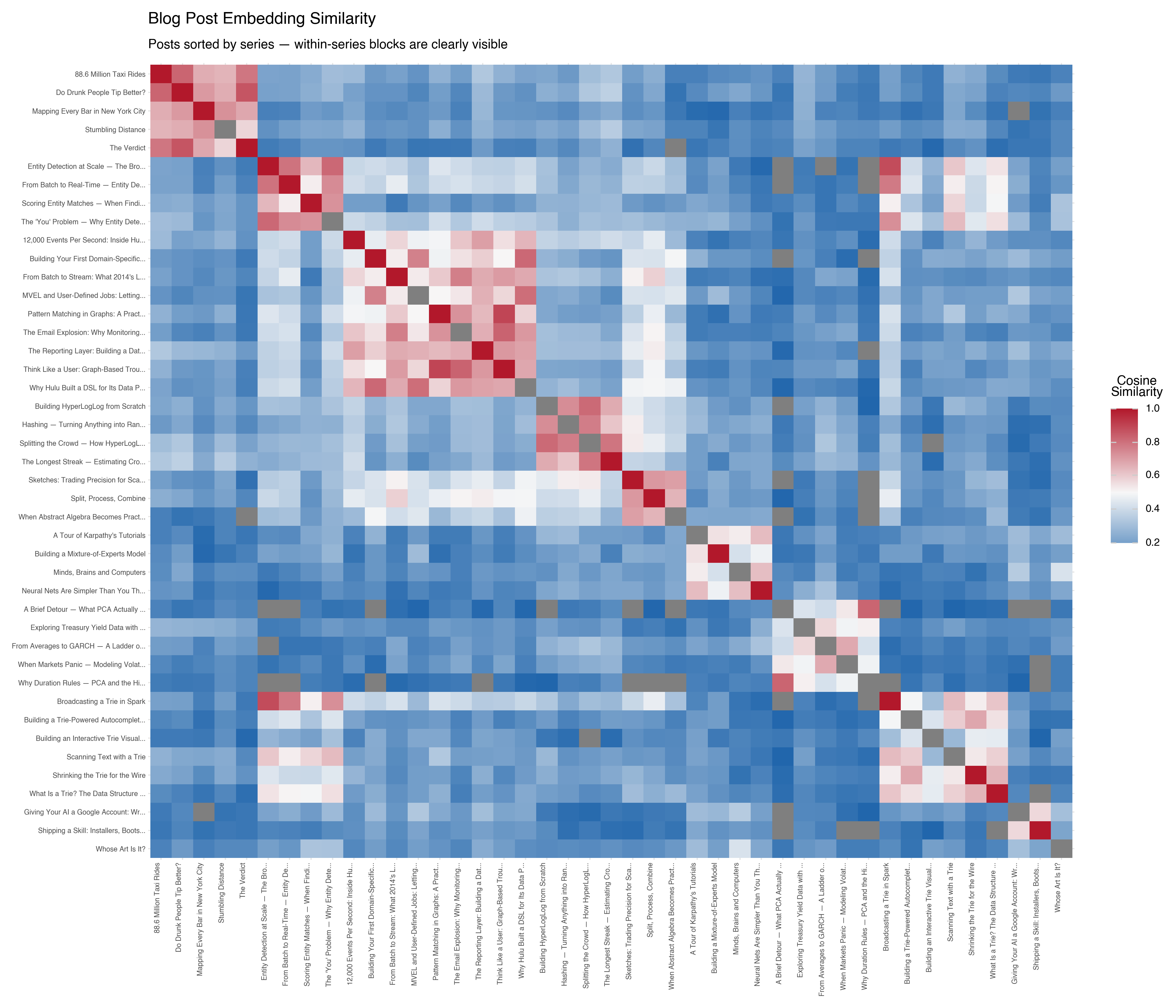
The block-diagonal structure leaps out. Posts in the same series form bright squares along the diagonal — the HyperLogLog posts are similar to each other, the neural nets posts cluster together, the Hulu pipeline posts form their own group.
But the interesting part is the off-diagonal structure. There’s a warm patch between the Entity Detection posts and the Tries posts — which makes sense, because my entity detection system uses tries for text scanning. The embeddings captured a relationship that exists in the content but isn’t reflected in the series labels.
We can also look at this as a distribution. If we separate all pairs into “same series” and “different series,” the picture is clear:
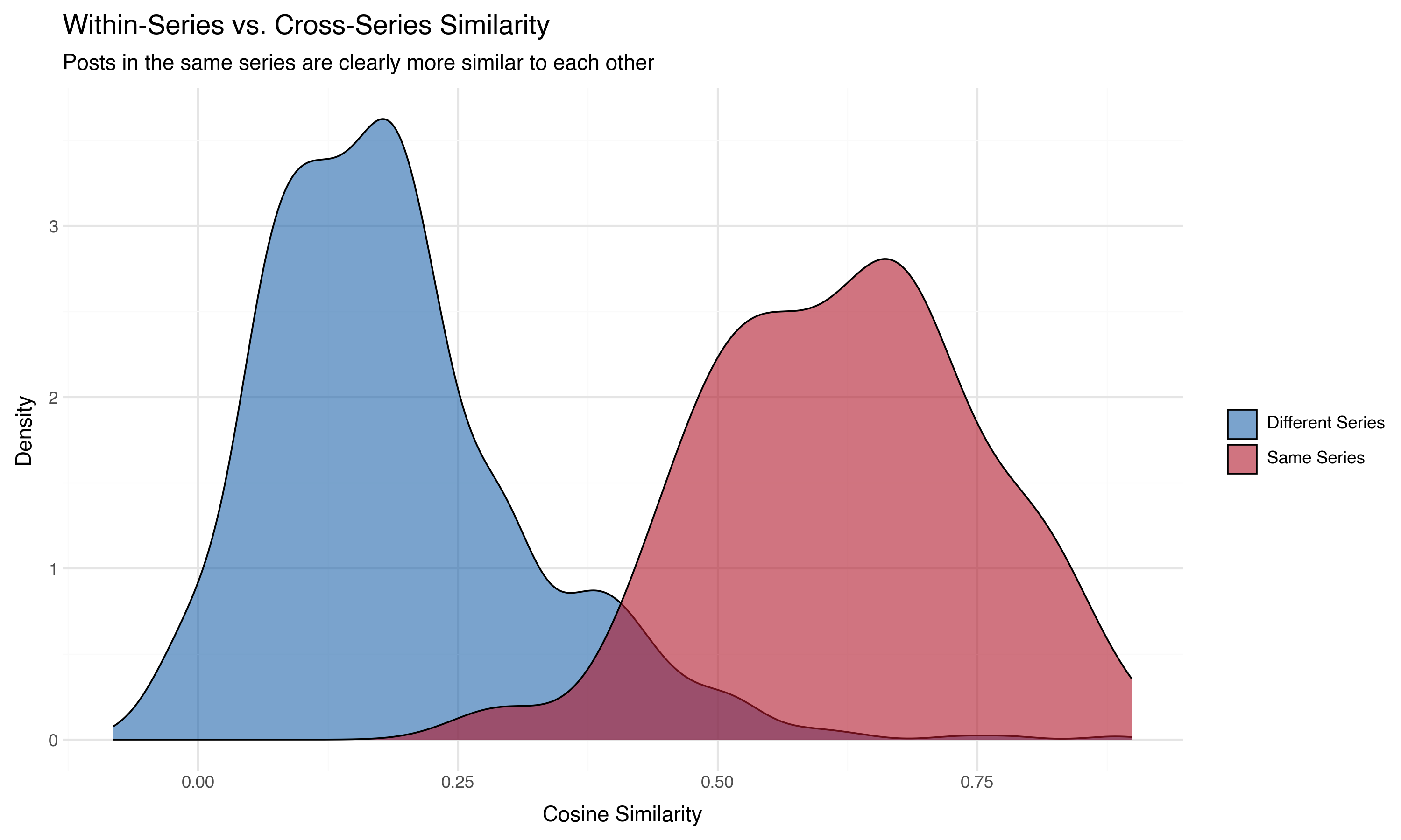
The mean similarity between posts in the same series is substantially higher than between posts in different series. The embeddings know which posts belong together, without ever being told about the series structure.
This is the hello world of embedding analysis. Forty-three documents, a pre-trained model, and ten lines of code — and we’ve recovered the topical structure of the blog.
The Speed-Accuracy Tradeoff: Bi-Encoders vs. Cross-Encoders
Everything we’ve done so far uses what’s called a bi-encoder: each text gets encoded independently into a vector, and we compare vectors with cosine similarity. This is fast — embed each document once, then compare any pair with a single dot product. It’s what makes embedding-based search possible over millions of documents.
But there’s a more accurate alternative: cross-encoders. Instead of encoding each text separately, a cross-encoder takes both texts as input simultaneously and produces a relevance score directly. The model can attend to the interaction between the two texts — spotting nuances that separate embeddings can’t capture.
The tradeoff is speed. A bi-encoder computes n embeddings for n documents, then any pair comparison is a dot product. A cross-encoder needs to run the full model for every pair — that’s O(n²). For 50,000 documents, that’s 1.25 billion model calls. Not practical.
The solution used in practice is retrieve-then-rerank: use embeddings (bi-encoder) to quickly narrow a large corpus to a shortlist of candidates, then use a cross-encoder to rerank just those candidates with higher accuracy.
from sentence_transformers import SentenceTransformer, CrossEncoder

# Step 1: Bi-encoder retrieval (fast, approximate)
bi_encoder = SentenceTransformer("all-mpnet-base-v2")
query_emb = bi_encoder.encode("a suspenseful thriller with an unexpected twist")
corpus_emb = bi_encoder.encode(movie_reviews)

# Cosine similarity to find top 20 candidates
scores = corpus_emb @ query_emb
top_20_indices = scores.argsort()[-20:][::-1]

# Step 2: Cross-encoder reranking (slow, precise)
cross_encoder = CrossEncoder("BAAI/bge-reranker-large")
pairs = [(query, movie_reviews[i]) for i in top_20_indices]
rerank_scores = cross_encoder.predict(pairs)

# The cross-encoder reshuffles the top 20 — its #1 is often
# different from the bi-encoder's #1, and usually better.
I used this pattern at Netflix to build a tool for finding the most relevant passage within a document. The bi-encoder found the right document; a cross-encoder (bge-reranker-large) then drilled down to the right paragraph. It worked by progressive narrowing — chunk the document into large pieces, cross-encode to find the best chunk, then re-chunk that winner into smaller pieces and cross-encode again, telescoping from document to paragraph to sentence.
The retrieve-then-rerank pattern shows up everywhere: search engines, RAG pipelines, recommendation systems. Embeddings get you in the neighborhood fast. Cross-encoders tell you exactly where to look.
Now What?
Here’s where it gets interesting — and where most embedding tutorials stop.
You’ve computed embeddings for your documents. You can compare them pairwise. You can find the most similar posts. It works. But we had 43 documents. What happens when you have 50,000?
For this series, we’re going to work with the Large Movie Review Dataset — 50,000 movie reviews from IMDB, split evenly between positive and negative sentiment, with star ratings from 1 to 10. We’ve embedded all of them into 768-dimensional vectors using the same all-mpnet-base-v2 model.
I chose entertainment data deliberately. I spent three years at Hulu building the data pipeline that powered their ad platform, and I’ve spent the past ten years at Netflix. I’ve worked with content metadata, user behavior signals, recommendation systems, and knowledge graphs built on entertainment data. When I look at movie review embeddings, I see familiar territory — and I know what questions are worth asking.
The questions that drive this series:
- What does the embedding space look like? Not the projection — the raw 768-dimensional space. What are the statistics? Is there structure, or is it noise? (Post 2)
- Can we see that structure? PCA, t-SNE, and UMAP each give a different view. What do they reveal, and what do they hide? (Post 3)
- Can we explore it interactively? A 3D data explorer built with Three.js, where you can fly through 10,000 movie reviews and understand the landscape. (Post 4)
- What are the clusters? If reviews group together, what do those groups mean? How do we go from “cluster 7” to “negative reviews of horror sequels”? (Post 5)
- What else can we learn? Embeddings aren’t the only signal. Genres, cast and crew networks, temporal patterns — feature engineering for high-dimensional data. (Post 6)
This is the workflow I’ve used in practice, and it’s the workflow this series follows: embed, explore, see, understand, enrich. Each post is a step in the process of making sense of a large dataset that lives in a space you can’t directly see.
But before we project or cluster anything, we need to look at the raw numbers. The next post starts with the question that should come first but almost never does: what does this data actually look like in 768 dimensions?
Key Takeaways
Embeddings are learned representations. A model processes text and produces a vector — a list of numbers — that captures semantic meaning. Words, sentences, or entire documents become points in a high-dimensional space.
Geometry encodes meaning. The direction between vectors captures relationships: gender, tense, geography, sentiment. These relationships emerge from patterns in how language is used, not from hand-coded rules.
Cosine similarity measures semantic distance. The angle between two embedding vectors tells you how similar their meaning is. This gives you a principled way to compare any two pieces of text.
Bi-encoders trade accuracy for speed; cross-encoders do the reverse. Embedding models (bi-encoders) encode texts independently — fast and scalable. Cross-encoders compare two texts jointly — more accurate but O(n²). Real systems use both: retrieve with embeddings, rerank with a cross-encoder.
Pre-trained models are the practical starting point. You don’t need to train your own embedding model (though you can). Open-source models via the sentence-transformers library, or API-based models from OpenAI and others, produce good general-purpose embeddings out of the box. The MTEB leaderboard tracks how they compare.
The interesting work starts after embedding. Getting the vectors is the easy part. Understanding what they tell you about your data is the series that follows.
Next: First Contact — Statistics and Distributions in High Dimensions