From Averages to GARCH — A Ladder of Time Series Models
In the first post, we found two inconvenient truths about Treasury yields: daily changes have fat tails and non-constant volatility. In the next post, we’ll use GARCH to model that volatility. But GARCH is a complicated-looking formula, and if you’re seeing it for the first time, it can feel like it dropped from the sky.
It didn’t. There’s a clean, intuitive ladder you can climb that makes GARCH feel almost inevitable rather than exotic. Each rung fixes a specific failure of the previous idea — which means you’re never adding complexity for its own sake. You’re adding it because something broke.
Let’s start at the bottom and climb.
Step 1: The Constant Mean — “Just Predict the Average”
Suppose you have a time series — daily Treasury yield changes, stock returns, temperature readings, whatever — and someone asks: what will tomorrow’s value be?
The simplest possible answer: predict the historical mean every single day.
import numpy as np
import matplotlib.pyplot as plt

# Simulate a simple series: daily changes with some structure
np.random.seed(42)
n = 300
true_values = np.cumsum(np.random.randn(n) * 0.5 + 0.02)

# "Model": predict the mean every day
prediction = np.full(n, true_values.mean())

fig, ax = plt.subplots(figsize=(10, 4))
ax.plot(true_values, color='#2c3e50', linewidth=0.8, label='Actual')
ax.axhline(true_values.mean(), color='#e74c3c', linestyle='--',
           linewidth=2, label=f'Constant mean = {true_values.mean():.2f}')
ax.set_title('Step 1: Predict the Mean', fontweight='bold')
ax.legend()
ax.grid(True, alpha=0.3)
plt.tight_layout()
plt.show()
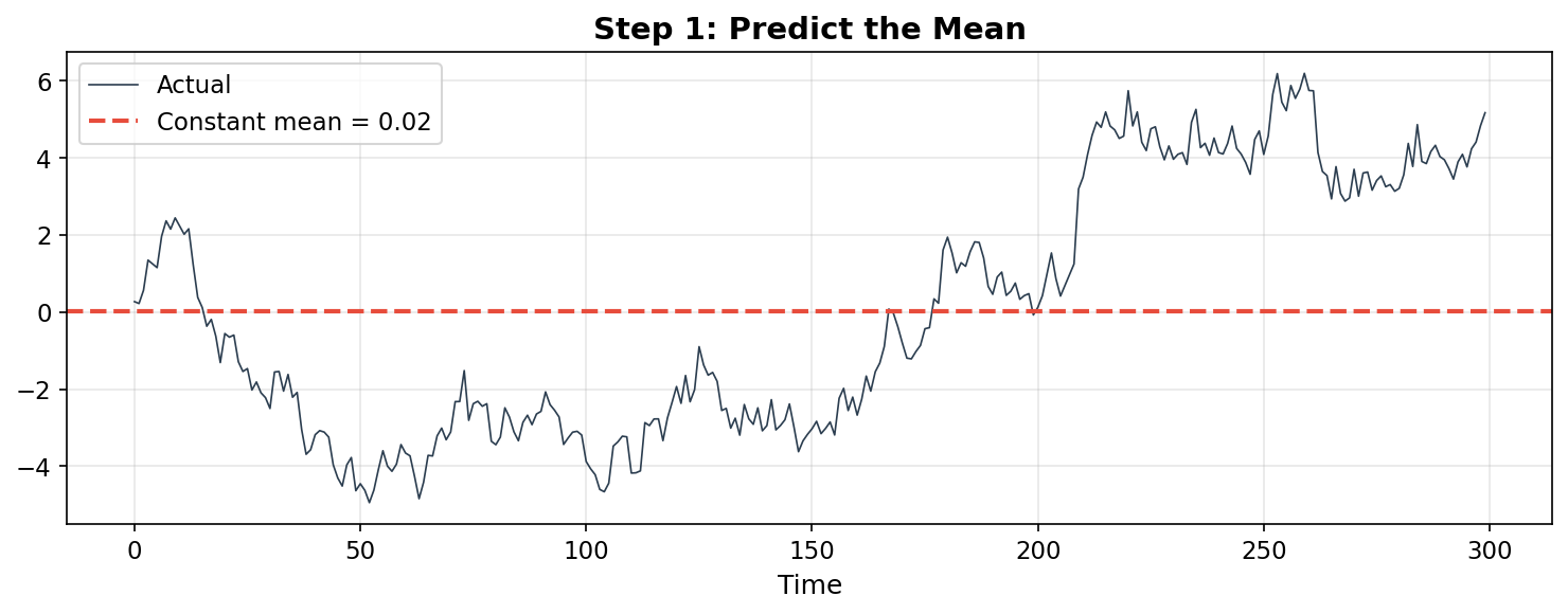
This is barely a model. It ignores everything — trends, momentum, recent history. The residuals (actual minus predicted) carry all the structure we threw away.
What breaks: The model ignores temporal structure entirely. Yesterday’s value tells you nothing — you predict the same number regardless. For a trending or autocorrelated series, this is useless.
What the next step fixes: Allow the prediction to depend on the past.
Step 2: White Noise — “The Mean Plus Random Shocks”
Before we add structure, let’s name what our constant-mean model implicitly assumes about the residuals: that they’re white noise — independent, identically distributed (i.i.d.) random draws with constant variance.
Formally:
x_t = μ + ε_t, where ε_t ~ N(0, σ²), i.i.d.
This says: the series is just a fixed mean plus random noise. No pattern, no memory, no clustering. Each day’s deviation from the mean is a coin flip, unrelated to yesterday’s.
# Generate actual white noise
white_noise = np.random.randn(300)

fig, axes = plt.subplots(1, 2, figsize=(12, 4))

# Time series plot
axes[0].plot(white_noise, color='#2c3e50', linewidth=0.5)
axes[0].set_title('White Noise: No Structure', fontweight='bold')
axes[0].axhline(0, color='gray', linestyle='--', alpha=0.5)

# Autocorrelation — should be zero at all lags
from statsmodels.graphics.tsaplots import plot_acf
plot_acf(white_noise, lags=20, ax=axes[1], color='#3498db')
axes[1].set_title('Autocorrelation: Flat', fontweight='bold')

plt.tight_layout()
plt.show()
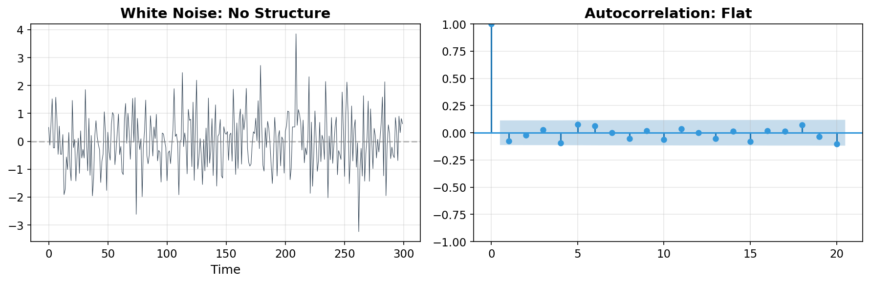
If your residuals look like this — no significant spikes in the autocorrelation function (ACF) — congratulations, there’s nothing left to model. But for most real-world financial time series, they don’t. The ACF shows significant spikes at short lags, meaning today’s value is correlated with yesterday’s.
What breaks: Real series have persistence — if yields went up yesterday, they’re somewhat more likely to go up (or down) today. White noise can’t capture this.
What the next step fixes: Let the current value depend on past values.
Step 3: AR(p) — “What Happened Recently Matters”
An autoregressive model of order p — AR(p) — says the current value is a linear combination of the previous p values, plus noise:
x_t = c + φ₁·x_{t-1} + φ₂·x_{t-2} + ... + φₚ·x_{t-p} + ε_t
The simplest version, AR(1), depends only on yesterday:
x_t = c + φ·x_{t-1} + ε_t
When |φ| < 1, the series is mean-reverting — it gets pulled back toward its average. When φ > 0, there’s positive persistence (momentum). When φ < 0, it oscillates.
from statsmodels.tsa.arima.model import ARIMA

# Simulate an AR(1) process with φ = 0.7
np.random.seed(42)
n = 300
ar_series = np.zeros(n)
phi = 0.7
for t in range(1, n):
    ar_series[t] = phi * ar_series[t-1] + np.random.randn()

# Fit AR(1) and inspect
model = ARIMA(ar_series, order=(1, 0, 0))
result = model.fit()
print(f"Estimated φ: {result.params[1]:.3f}  (true: {phi})")

fig, axes = plt.subplots(1, 2, figsize=(12, 4))
axes[0].plot(ar_series, color='#2c3e50', linewidth=0.7)
axes[0].set_title(f'AR(1) with φ={phi}: Persistent', fontweight='bold')

residuals = result.resid
plot_acf(residuals, lags=20, ax=axes[1], color='#27ae60')
axes[1].set_title('Residual ACF: Much Better', fontweight='bold')

plt.tight_layout()
plt.show()
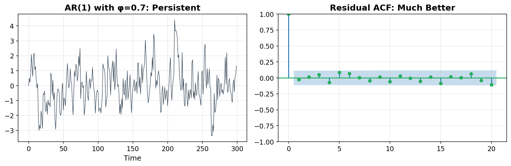
The AR model captures the mean dynamics — the tendency for the series to drift and revert. After fitting, the residuals should have much less autocorrelation.
What breaks: AR captures dependence on past values, but sometimes the series also depends on past shocks — events that temporarily perturbed the series but whose direct effect fades. Also, AR still assumes constant variance in the noise term.
What the next step fixes: Model the shocks directly.
Step 4: MA(q) — “Past Shocks Leave Echoes”
A moving average model of order q — MA(q) — says the current value depends on the past shocks (errors) rather than past values:
x_t = μ + ε_t + θ₁·ε_{t-1} + θ₂·ε_{t-2} + ... + θ_q·ε_{t-q}
Think of it this way: an AR model says “where the series is predicts where it goes.” An MA model says “the shocks that hit the series leave echoes for a few periods.”
In practice, the distinction matters less than you might think — many series can be modeled equally well by either AR or MA. But sometimes one gives a more parsimonious (fewer parameter) fit than the other. And combining them gives us the best of both worlds.
What breaks: Neither AR nor MA alone is always the most efficient model. And both still assume constant variance.
What the next step fixes: Combine them.
Step 5: ARMA(p,q) — “The Best of Both Worlds”
ARMA simply combines the AR and MA components:
x_t = c + φ₁·x_{t-1} + ... + φₚ·x_{t-p} + ε_t + θ₁·ε_{t-1} + ... + θ_q·ε_{t-q}
This is the workhorse of stationary time series modeling. The AR part captures persistence in levels; the MA part captures the decay of shock effects. Together, they can approximate a wide variety of autocorrelation structures with relatively few parameters.
For a software engineer, think of it as a PID controller for time series: the AR part is like the proportional term (responding to where you are), and the MA part is like the derivative term (responding to recent disturbances).
What breaks: ARMA assumes the series is stationary — no trends, no unit roots. If the series is drifting upward or downward over time, ARMA gives nonsensical results.
What the next step fixes: Handle non-stationarity.
Step 6: ARIMA(p,d,q) — “Difference Away the Trends”
The “I” in ARIMA stands for “Integrated.” The idea is simple: if the series has a trend, difference it (subtract each value from the previous one) until it’s stationary, then fit ARMA to the differenced series.
ARIMA(p, d, q): Apply d differences, then fit ARMA(p, q)
For Treasury yields, we’ve been working with daily changes (first differences) since the beginning of this series — that’s exactly d=1 differencing. The raw yield level has a trend; the daily changes are roughly stationary.
# Example: raw series with a trend vs. differenced series
np.random.seed(42)
n = 300
trend_series = np.cumsum(np.random.randn(n) * 0.5 + 0.1)  # upward drift
differenced = np.diff(trend_series)

fig, axes = plt.subplots(1, 2, figsize=(12, 4))
axes[0].plot(trend_series, color='#8e44ad', linewidth=0.8)
axes[0].set_title('Non-Stationary: Trending Up', fontweight='bold')

axes[1].plot(differenced, color='#27ae60', linewidth=0.5)
axes[1].axhline(0, color='gray', linestyle='--', alpha=0.5)
axes[1].set_title('After Differencing: Stationary', fontweight='bold')

plt.tight_layout()
plt.show()
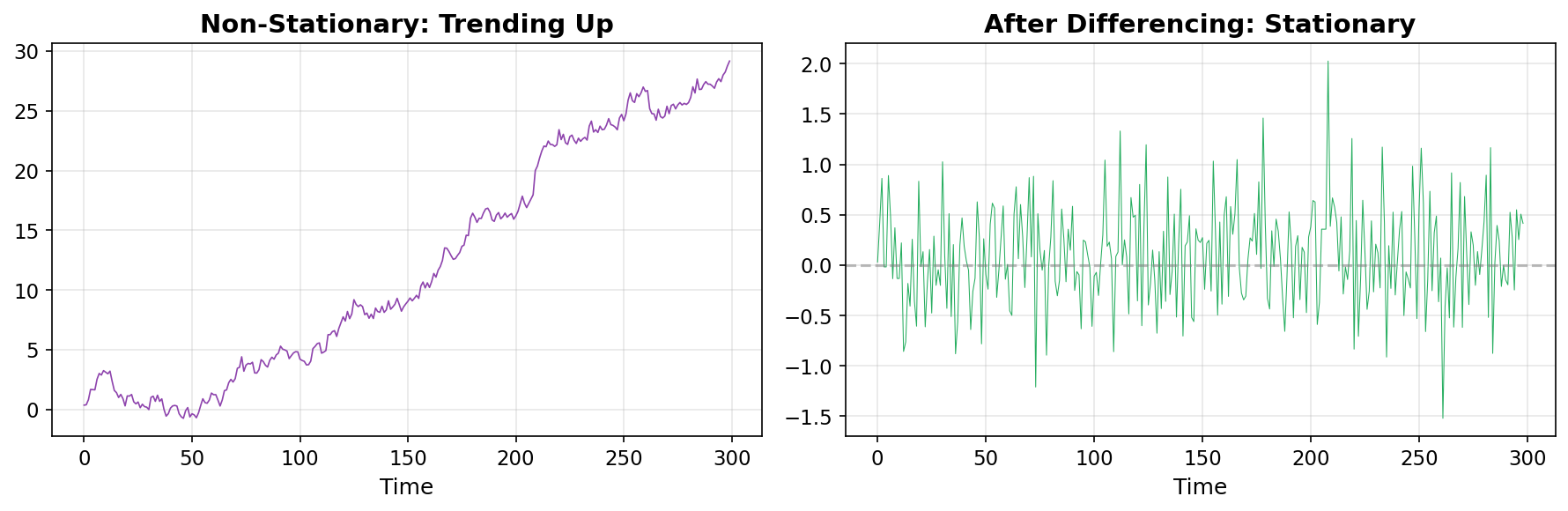
ARIMA handles the full pipeline: remove trends via differencing, then model the remaining structure with AR and MA terms. For most applications, d=1 (one round of differencing) is enough.
What breaks: ARIMA models the mean of the series beautifully. But it still assumes the variance of the noise is constant. Look at the residuals from any ARIMA fit to financial data and you’ll see periods of big noise and periods of small noise. The errors are heteroskedastic — their spread changes over time.
This is exactly the volatility clustering we discovered in the first post.
What the next step fixes: Model the variance itself as a time-varying process.
The Pivot: When Variance Isn’t Constant
This is the key moment in the ladder. Let me show you why everything above breaks down for financial data.
Take a well-fitted ARIMA model. Extract the residuals. If the model captured all the structure, these residuals should be white noise — boring, featureless, constant variance. Let’s check:
# Simulate a series with volatility clustering (what real data looks like)
np.random.seed(42)
n = 1000
vol = np.ones(n) * 1.0
for t in range(1, n):
    vol[t] = np.sqrt(0.05 + 0.1 * (np.random.randn()**2) + 0.85 * vol[t-1]**2)
returns = vol * np.random.randn(n)

# Fit ARIMA(1,0,1) — captures the mean dynamics
model = ARIMA(returns, order=(1, 0, 1))
result = model.fit()
residuals = result.resid

fig, axes = plt.subplots(2, 2, figsize=(12, 8))

# Top left: residuals look OK at first glance
axes[0, 0].plot(residuals, color='#2c3e50', linewidth=0.5)
axes[0, 0].set_title('Residuals: Look OK?', fontweight='bold')

# Top right: but the squared residuals show clustering!
axes[0, 1].plot(residuals**2, color='#e74c3c', linewidth=0.5)
axes[0, 1].set_title('Squared Residuals: Clustered!', fontweight='bold')

# Bottom left: ACF of residuals — fine
plot_acf(residuals, lags=20, ax=axes[1, 0], color='#3498db')
axes[1, 0].set_title('ACF of Residuals: Clean', fontweight='bold')

# Bottom right: ACF of SQUARED residuals — significant autocorrelation!
plot_acf(residuals**2, lags=20, ax=axes[1, 1], color='#e74c3c')
axes[1, 1].set_title('ACF of Squared Residuals: Structured!', fontweight='bold')

plt.tight_layout()
plt.show()
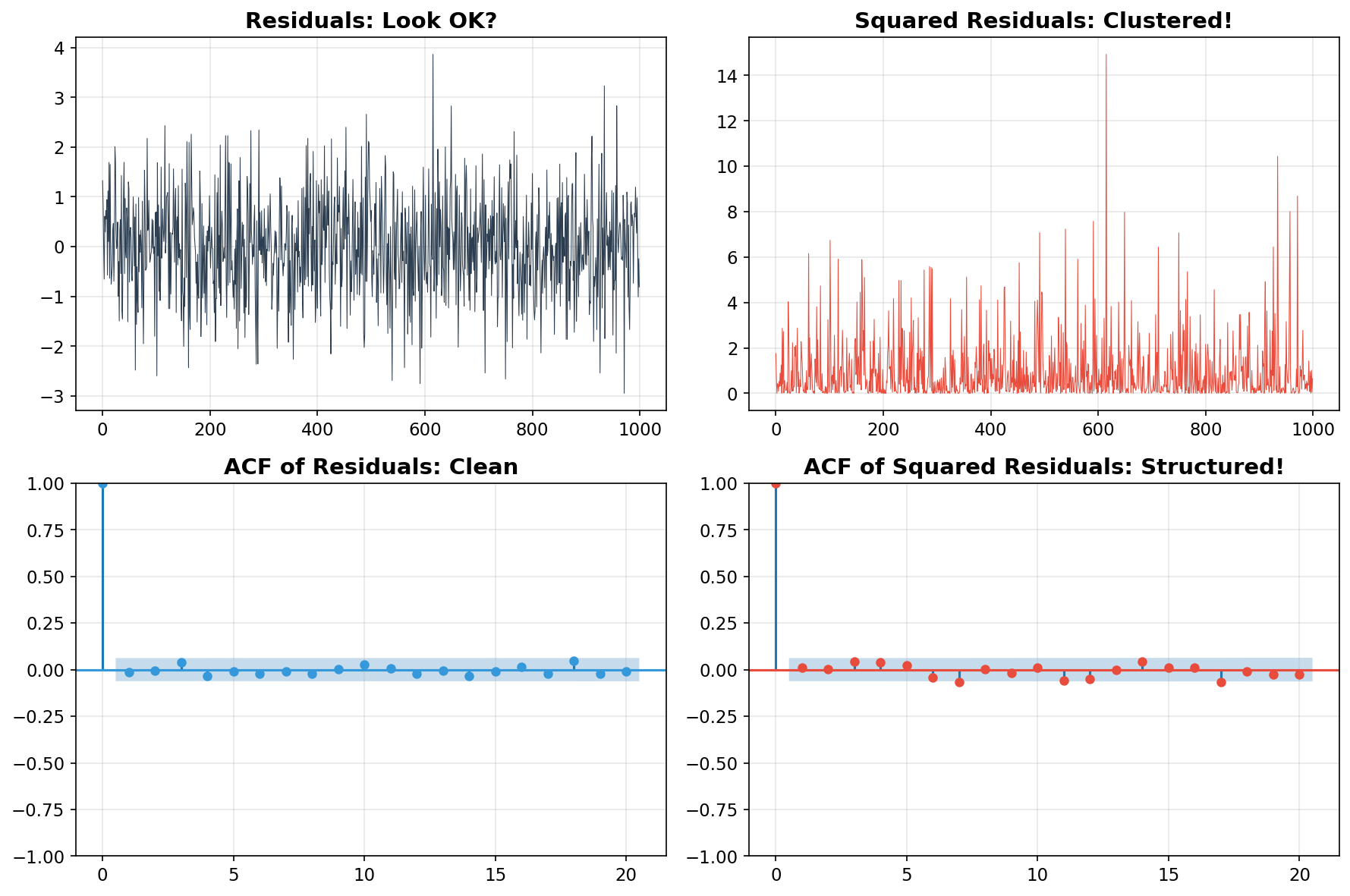
The top-left panel looks fine — the residuals bounce around zero with no obvious pattern. The bottom-left ACF confirms no autocorrelation in the residuals themselves.
But look at the squared residuals (top-right): they cluster! Big residuals are followed by big residuals, small by small. The ACF of squared residuals (bottom-right) shows strong, slowly decaying autocorrelation.
This means: the ARIMA model got the mean right, but the variance of the noise is predictable. Volatility itself is a structured, forecastable process. That’s the insight that Robert Engle won the Nobel Prize for, and it’s what the next two models capture.
Step 7: ARCH(q) — “Volatility Depends on Recent Shocks”
ARCH — Autoregressive Conditional Heteroskedasticity — is the breakthrough. Instead of modeling the level of the series, ARCH models the variance of the noise:
σ²_t = ω + α₁·ε²_{t-1} + α₂·ε²_{t-2} + ... + α_q·ε²_{t-q}
In plain English: today’s expected variance is a baseline (ω) plus a weighted sum of recent squared surprises. If yesterday had a big shock (large ε²), today’s variance goes up. If yesterday was calm, variance stays low.
The simplest case, ARCH(1):
σ²_t = ω + α·ε²_{t-1}
from arch import arch_model

# Fit an ARCH(3) model — variance depends on last 3 squared shocks
am = arch_model(returns, vol='ARCH', p=3, mean='zero')
res = am.fit(disp='off')

print("ARCH(3) parameters:")
print(f"  ω (baseline):   {res.params['omega']:.4f}")
for i in range(1, 4):
    print(f"  α{i} (lag {i}):     {res.params[f'alpha[{i}]']:.4f}")

fig, ax = plt.subplots(figsize=(10, 4))
ax.plot(res.conditional_volatility, color='#e67e22', linewidth=0.8,
        label='ARCH(3) Conditional Volatility')
ax.set_title('ARCH: Variance Responds to Shocks', fontweight='bold')
ax.legend()
ax.grid(True, alpha=0.3)
plt.tight_layout()
plt.show()
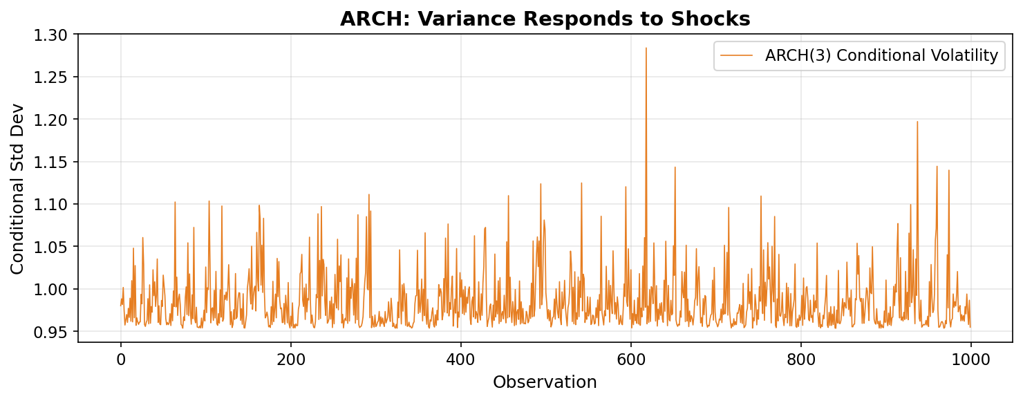
ARCH is a genuine breakthrough — it formalizes the idea that volatility is predictable. But it has a limitation: since it only looks at a fixed window of past shocks (the last q days), it has short memory. If you want to capture the kind of slow-decay persistence we see in real volatility — where a crisis keeps markets jittery for months — you’d need a very high q, which means estimating many parameters.
What breaks: Short memory. To capture persistent volatility (the kind that decays over weeks or months), you need many lags, which means many parameters. The model becomes unwieldy and unstable.
What the next step fixes: Give volatility its own momentum — let it persist without needing dozens of explicit lags.
Step 8: GARCH(p,q) — “Volatility Has Memory”
GARCH — Generalized ARCH — adds a simple but powerful extension: the variance depends not only on past shocks, but also on its own past values:
σ²_t = ω + α·ε²_{t-1} + β·σ²_{t-1}
That extra term β·σ²_{t-1} is the magic. It gives volatility momentum — if yesterday’s volatility was high, today’s will be too, even if yesterday’s actual shock was small. This creates the slow, persistent decay we observe in real markets: a crisis doesn’t just spike volatility for one day, it keeps it elevated for weeks or months.
The recursion in β·σ²_{t-1} means that GARCH(1,1) effectively captures an infinite history of past shocks with just three parameters (ω, α, β). Compare that to ARCH, where you’d need dozens of lag terms to achieve the same persistence.
# Fit GARCH(1,1) — the gold standard
am_garch = arch_model(returns, vol='GARCH', p=1, q=1, mean='zero')
res_garch = am_garch.fit(disp='off')

alpha = res_garch.params['alpha[1]']
beta = res_garch.params['beta[1]']

print("GARCH(1,1) parameters:")
print(f"  ω (baseline):    {res_garch.params['omega']:.4f}")
print(f"  α (shock weight): {alpha:.4f}")
print(f"  β (persistence):  {beta:.4f}")
print(f"  α + β:            {alpha + beta:.4f}")

if alpha + beta < 1:
    halflife = np.log(2) / -np.log(alpha + beta)
    print(f"  Half-life:        {halflife:.0f} periods")

fig, ax = plt.subplots(figsize=(10, 4))
ax.plot(res.conditional_volatility, color='#e67e22', linewidth=0.6,
        alpha=0.6, label='ARCH(3)')
ax.plot(res_garch.conditional_volatility, color='#8e44ad', linewidth=1.2,
        label='GARCH(1,1)')
ax.set_title('ARCH vs. GARCH: Persistence Matters', fontweight='bold')
ax.legend()
ax.grid(True, alpha=0.3)
plt.tight_layout()
plt.show()
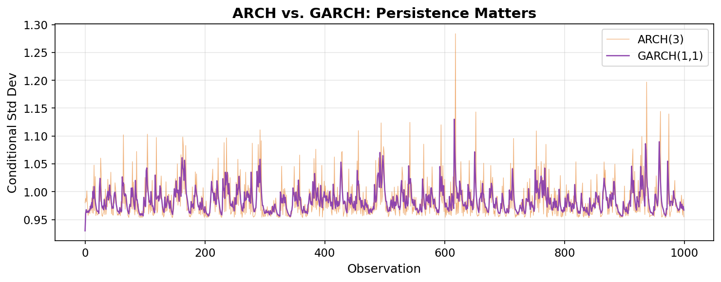
GARCH(1,1) is the most widely used volatility model in finance. For Treasury yields, typical values are α ≈ 0.05 and β ≈ 0.94, giving α + β ≈ 0.99 — meaning volatility is extremely persistent. After a shock, it takes roughly 70 days for volatility to decay halfway back to its long-run level.
The Complete Ladder
Here’s the full progression, laid out as a table:
| Step | Model | What it assumes | What breaks | What the next step fixes |
|---|---|---|---|---|
| 1 | Constant Mean | Series fluctuates around a fixed mean | Ignores temporal structure | Allow dependence on the past |
| 2 | White Noise | Mean + i.i.d. noise with constant variance | No persistence or predictability | Model autocorrelation |
| 3 | AR(p) | Current value depends on past values | Doesn’t capture shock echoes | Model shocks directly |
| 4 | MA(q) | Current value depends on past shocks | Often needs to be combined with AR | Combine level + shock dynamics |
| 5 | ARMA(p,q) | Past values and past shocks matter | Can’t handle trends | Allow non-stationary series |
| 6 | ARIMA(p,d,q) | Differencing removes trends | Assumes constant variance | Model changing variance |
| 7 | ARCH(q) | Variance depends on recent shocks | Short-memory volatility | Add persistent volatility |
| 8 | GARCH(p,q) | Variance depends on past variance and shocks | — | Persistent, clustered volatility |
The intuition thread
- AR → ARMA → ARIMA fix progressively harder problems with the mean.
- ARCH says: “volatility itself is predictable.”
- GARCH says: “and volatility has memory.”
Each step exists because the previous one failed in a specific, observable way. Nobody sat down and invented GARCH from scratch — it was the natural endpoint of decades of researchers looking at residuals, seeing structure, and building models to capture it.
Further Reading
If you want to go deeper into the time series foundations behind this ladder, here are the books I’d recommend:
To expand on the intuition:
- Chatfield, Chris, The Analysis of Time Series: An Introduction — Classic introduction. Chatfield covers everything from AR through ARIMA with exceptional clarity and a focus on building intuition before formalism.
- Janacek, Gareth, Practical Time Series — More concise and applied than Chatfield, but still practical and not too heavy on proofs.
To dive deeper into the math:
- Hamilton, James D., Time Series Analysis — The graduate-level reference. Comprehensive and rigorous — covers everything from basic ARMA theory through state-space models and GARCH. Heavy going, but definitive. This is the book you reach for when the others don’t go deep enough.
Specific to finance:
- Tsay, Ruey S., Analysis of Financial Time Series — Bridges the gap between general time series and financial applications. Tsay covers ARMA, GARCH, and their many extensions with financial examples throughout. If you’re specifically interested in the finance side, this is the most directly relevant.
These are the original papers that introduced the concepts:
- Engle, Robert F. (1982), “Autoregressive Conditional Heteroskedasticity with Estimates of the Variance of United Kingdom Inflation” — The original ARCH paper. Readable and surprisingly accessible for an econometrics paper.
- Bollerslev, Tim (1986), “Generalized Autoregressive Conditional Heteroskedasticity” — The paper that generalized ARCH to GARCH. Short and to the point.
What’s Next
Now that you know why GARCH exists and where it sits in the landscape of time series models, we’re ready to apply it. In the next post, we’ll fit GARCH(1,1) to 30 years of Treasury yield data, build a dynamic VaR envelope, and investigate which historical crises show up as extreme moves.